Figure 13.1
Table of contents
At the end of this chapter you should be able to:
Describe the nature of transactions and the reasons for designing database systems around transactions.
Explain the causes of transaction failure.
Analyse the problems of data management in a concurrent environment.
Critically compare the relative strengths of different concurrency control approaches.
In parallel with this chapter, you should read Chapter 20 of Thomas Connolly and Carolyn Begg, "Database Systems A Practical Approach to Design, Implementation, and Management", (5th edn.).
The purpose of this chapter is to introduce the fundamental technique of concurrency control, which provides database systems with the ability to handle many users accessing data simultaneously. In addition, this chapter helps you understand the functionality of database management systems, with special reference to online transaction processing (OLTP). The chapter also describes the problems that arise out of the fact that users wish to query and update stored data at the same time, and the approaches developed to address these problems, together with their respective strengths and weaknesses in a range of practical situations.
There are a number of concepts that are technical and unfamiliar. You will be expected to be able to handle these concepts but not to have any knowledge of the detailed algorithms involved. This chapter fits closely with the one on backup and recovery, so you may want to revisit this chapter later in the course to review the concepts. It will become clear from the information on concurrency control that there are a number of circumstances where recovery procedures may need to be invoked to salvage previous or currently executing transactions. The material covered here will be further extended in the chapter on distributed database systems, where we shall see how effective concurrency control can be implemented across a computer network.
Many criteria can be used to classify DBMSs, one of which is the number of users supported by the system. Single-user systems support only one user at a time and are mostly used with personal computers. Multi-user systems, which include the majority of DBMSs, support many users concurrently.
In this chapter, we will discuss the concurrency control problem, which occurs when multiple transactions submitted by various users interfere with one another in a way that produces incorrect results. We will start the chapter by introducing some basic concepts of transaction processing. Why concurrency control and recovery are necessary in a database system is then discussed. The concept of an atomic transaction and additional concepts related to transaction processing in database systems are introduced. The concepts of atomicity, consistency, isolation and durability – the so-called ACID properties that are considered desirable in transactions - are presented.
The concept of schedules of executing transactions and characterising the recoverability of schedules is introduced, with a detailed discussion of the concept of serialisability of concurrent transaction executions, which can be used to define correct execution sequences of concurrent transactions.
We will also discuss recovery from transaction failures. A number of concurrency control techniques that are used to ensure noninterference or isolation of concurrently executing transactions are discussed. Most of these techniques ensure serialisability of schedules, using protocols or sets of rules that guarantee serialisability. One important set of protocols employs the technique of locking data items, to prevent multiple transactions from accessing the items concurrently. Another set of concurrency control protocols use transaction timestamps. A timestamp is a unique identifier for each transaction generated by the system. Concurrency control protocols that use locking and timestamp ordering to ensure serialisability are both discussed in this chapter.
An overview of recovery techniques will be presented in a separate chapter.
The first concept that we introduce to you in this chapter is a transaction. A transaction is the execution of a program that accesses or changes the contents of a database. It is a logical unit of work (LUW) on the database that is either completed in its entirety (COMMIT) or not done at all. In the latter case, the transaction has to clean up its own mess, known as ROLLBACK. A transaction could be an entire program, a portion of a program or a single command.
The concept of a transaction is inherently about organising functions to manage data. A transaction may be distributed (available on different physical systems or organised into different logical subsystems) and/or use data concurrently with multiple users for different purposes.
Online transaction processing (OLTP) systems support a large number of concurrent transactions without imposing excessive delays.
For recovery purposes, a system always keeps track of when a transaction starts, terminates, and commits or aborts. Hence, the recovery manager keeps track of the following transaction states and operations:
BEGIN_TRANSTRACTION: This marks the beginning of transaction execution.
READ or WRITE: These specify read or write operations on the database items that are executed as part of a transaction.
END_TRANSTRACTION: This specifies that read and write operations have ended and marks the end limit of transaction execution. However, at this point it may be necessary to check whether the changes introduced by the transaction can be permanently applied to the database (committed) or whether the transaction has to be aborted because it violates concurrency control, or for some other reason (rollback).
COMMIT_TRANSTRACTION: This signals a successful end of the transaction so that any changes (updates) executed by the transaction can be safely committed to the database and will not be undone.
ROLLBACK (or ABORT): This signals the transaction has ended unsuccessfully, so that any changes or effects that the transaction may have applied to the database must be undone.
In addition to the preceding operations, some recovery techniques require additional operations that include the following:
UNDO: Similar to rollback, except that it applies to a single operation rather than to a whole transaction.
REDO: This specifies that certain transaction operations must be redone to ensure that all the operations of a committed transaction have been applied successfully to the database.
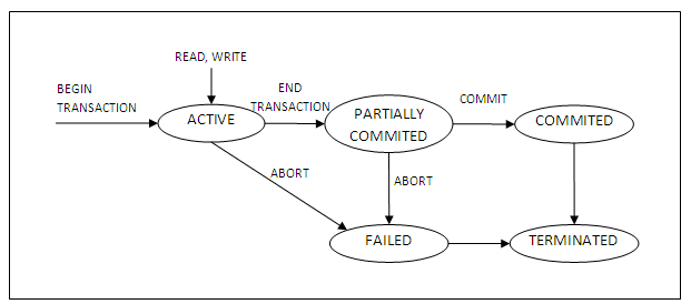
A state transaction diagram is shown below:
Figure 13.1
It shows clearly how a transaction moves through its execution states. In the diagram, circles depict a particular state; for example, the state where a transaction has become active. Lines with arrows between circles indicate transitions or changes between states; for example, read and write, which correspond to computer processing of the transaction.
A transaction goes into an active state immediately after it starts execution, where it can issue read and write operations. When the transaction ends, it moves to the partially committed state. At this point, some concurrency control techniques require that certain checks be made to ensure that the transaction did not interfere with other executing transactions. In addition, some recovery protocols are needed to ensure that a system failure will not result in inability to record the changes of the transaction permanently. Once both checks are successful, the transaction is said to have reached its commit point and enters the committed state. Once a transaction enters the committed state, it has concluded its execution successfully.
However, a transaction can go to the failed state if one of the checks fails or if it aborted during its active state. The transaction may then have to be rolled back to undo the effect of its write operations on the database. The terminated state corresponds to the transaction leaving the system. Failed or aborted transactions may be restarted later, either automatically or after being resubmitted, as brand new transactions.
Many computer systems, including DBMSs, are used simultaneously by more than one user. This means the computer runs multiple transactions (programs) at the same time. For example, an airline reservations system is used by hundreds of travel agents and reservation clerks concurrently. Systems in banks, insurance agencies, stock exchanges and the like are also operated by many users who submit transactions concurrently to the system. If, as is often the case, there is only one CPU, then only one program can be processed at a time. To avoid excessive delays, concurrent systems execute some commands from one program (transaction), then suspended that program and execute some commands from the next program, and so on. A program is resumed at the point where it was suspended when it gets its turn to use the CPU again. This is known as interleaving.
The figure below shows two programs A and B executing concurrently in an interleaved fashion. Interleaving keeps the CPU busy when an executing program requires an input or output (I/O) operation, such as reading a block of data from disk. The CPU is switched to execute another program rather than remaining idle during I/O time.
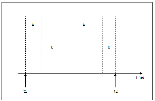
Figure 13.2
If the computer system has multiple hardware processors (CPUs), simultaneous processing of multiple programs is possible, leading to simultaneous rather than interleaved concurrency, as illustrated by program C and D in the figure below. Most of the theory concerning concurrency control in databases is developed in terms of interleaved concurrency, although it may be adapted to simultaneous concurrency.
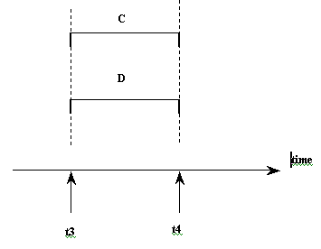
Figure 13.3
Concurrency is the ability of the database management system to process more than one transaction at a time. You should distinguish genuine concurrency from the appearance of concurrency. The database management system may queue transactions and process them in sequence. To the users it will appear to be concurrent but for the database management system it is nothing of the kind. This is discussed under serialisation below.
We deal with transactions at the level of data items and disk blocks for the purpose of discussing concurrency control and recovery techniques. At this level, the database access operations that a transaction can include are:
read_item(X): Reads a database item named X into a program variable also named X.
write_item(X): Writes the value of program variable X into the database item named X.
Executing a read_item(X) command includes the following steps:
Find the address of the disk block that contains item X.
Copy the disk block into a buffer in main memory if that disk is not already in some main memory buffer.
Copy item X from the buffer to the program variable named X.
Executing a write_item(X) command includes the following steps:
Find the address of the disk block that contains item X.
Copy the disk block into a buffer in main memory if that disk is not already in some main memory buffer.
Copy item X from the program variable named X into its correct location in the buffer.
Store the updated block from the buffer back to disk (either immediately or at some later point in time).
Step 4 is the one that actually updates the database on disk. In some cases the buffer is not immediately stored to disk, in case additional changes are to be made to the buffer. Usually, the decision about when to store back a modified disk block that is in a main memory buffer is handled by the recovery manager or the operating system.
A transaction will include read and write operations to access the database. The figure below shows examples of two very simple transactions. Concurrency control and recovery mechanisms are mainly concerned with the database access commands in a transaction.
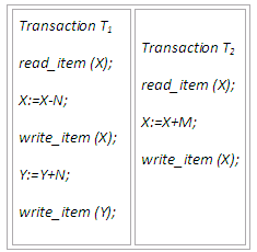
Figure 13.4
The above two transactions submitted by any two different users may be executed concurrently and may access and update the same database items (e.g. X). If this concurrent execution is uncontrolled, it may lead to problems such as an inconsistent database. Some of the problems that may occur when concurrent transactions execute in an uncontrolled manner are discussed in the next section.
Activity 1 - Looking up glossary entries
In the Concurrent Access to Data section of this chapter, the following phrases have glossary entries:
transaction
interleaving
COMMIT
ROLLBACK
In your own words, write a short definition for each of these terms.
Look up and make notes of the definition of each term in the module glossary.
Identify (and correct) any important conceptual differences between your definition and the glossary entry.
Review question 1
Explain what is meant by a transaction. Discuss the meaning of transaction states and operations.
In your own words, write the key feature(s) that would distinguish an interleaved concurrency from a simultaneous concurrency.
Use an example to illustrate your point(s) given in 2.
Discuss the actions taken by the read_item and write_item operations on a database.
Concurrency is the ability of the DBMS to process more than one transaction at a time. This section briefly overviews several problems that can occur when concurrent transactions execute in an uncontrolled manner. Concrete examples are given to illustrate the problems in details. The related activities and learning tasks that follow give you a chance to evaluate the extent of your understanding of the problems. An important learning objective for this section of the chapter is to understand the different types of problems of concurrent executions in OLTP, and appreciate the need for concurrency control.
We illustrate some of the problems by referring to a simple airline reservation database in which each record is stored for each airline flight. Each record includes the number of reserved seats on that flight as a named data item, among other information. Recall the two transactions T1 and T2 introduced previously:
Figure 13.5
Transaction T1 cancels N reservations from one flight, whose number of reserved seats is stored in the database item named X, and reserves the same number of seats on another flight, whose number of reserved seats is stored in the database item named Y. A simpler transaction T2 just reserves M seats on the first flight referenced in transaction T1. To simplify the example, the additional portions of the transactions are not shown, such as checking whether a flight has enough seats available before reserving additional seats.
When an airline reservation database program is written, it has the flight numbers, their dates and the number of seats available for booking as parameters; hence, the same program can be used to execute many transactions, each with different flights and number of seats to be booked. For concurrency control purposes, a transaction is a particular execution of a program on a specific date, flight and number of seats. The transactions T1 and T2 are specific executions of the programs that refer to the specific flights whose numbers of seats are stored in data item X and Y in the database. Now let’s discuss the types of problems we may encounter with these two transactions.
The lost update problem occurs when two transactions that access the same database items have their operations interleaved in a way that makes the value of some database item incorrect. That is, interleaved use of the same data item would cause some problems when an update operation from one transaction overwrites another update from a second transaction.
An example will explain the problem clearly. Suppose the two transactions T1 and T2 introduced previously are submitted at approximately the same time. It is possible when two travel agency staff help customers to book their flights at more or less the same time from a different or the same office. Suppose that their operations are interleaved by the operating system as shown in the figure below:
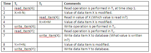
Figure 13.6
The above interleaved operation will lead to an incorrect value for data item X, because at time step 3, T2 reads in the original value of X which is before T1 changes it in the database, and hence the updated value resulting from T1 is lost. For example, if X = 80, originally there were 80 reservations on the flight, N = 5, T1 cancels 5 seats on the flight corresponding to X and reserves them on the flight corresponding to Y, and M = 4, T2 reserves 4 seats on X.
The final result should be X = 80 – 5 + 4 = 79; but in the concurrent operations of the figure above, it is X = 84 because the update that cancelled 5 seats in T1 was lost.
The detailed value updating in the flight reservation database in the above example is shown below:
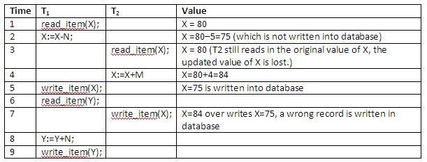
Figure 13.7
Uncommitted dependency occurs when a transaction is allowed to retrieve or (worse) update a record that has been updated by another transaction, but which has not yet been committed by that other transaction. Because it has not yet been committed, there is always a possibility that it will never be committed but rather rolled back, in which case, the first transaction will have used some data that is now incorrect - a dirty read for the first transaction.
The figure below shows an example where T1 updates item X and then fails before completion, so the system must change X back to its original value. Before it can do so, however, transaction T2 reads the 'temporary' value of X, which will not be recorded permanently in the database because of the failure of T1. The value of item X that is read by T2 is called dirty data, because it has been created by a transaction that has not been completed and committed yet; hence this problem is also known as the dirty read problem. Since the dirty data read in by T2 is only a temporary value of X, the problem is sometimes called temporary update too.
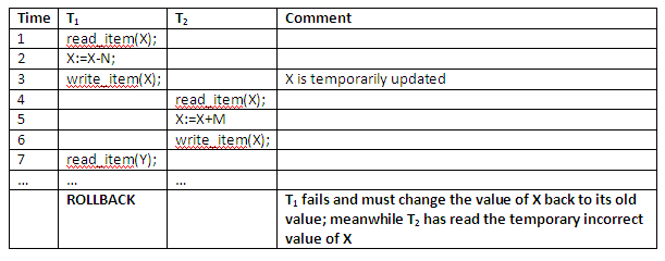
Figure 13.8
The rollback of transaction T1 may be due to a system crash, and transaction T2 may already have terminated by that time, in which case the crash would not cause a rollback to be issued for T2. The following situation is even more unacceptable:
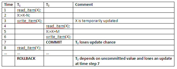
Figure 13.9
In the above example, not only does transaction T2 becomes dependent on an uncommitted change at time step 6, but it also loses an update at time step 7, because the rollback in T1 causes data item X to be restored to its value before time step 1.
Inconsistent analysis occurs when a transaction reads several values, but a second transaction updates some of these values during the execution of the first. This problem is significant, for example, if one transaction is calculating an aggregate summary function on a number of records while other transactions are updating some of these records. The aggregate function may calculate some values before they are updated and others after they are updated. This causes an inconsistency.
For example, suppose that a transaction T3 is calculating the total number of reservations on all the flights; meanwhile, transaction T1 is executing. If the interleaving of operations shown below occurs, the result of T3 will be off by amount N, because T3 reads the value of X after N seats have been subtracted from it, but reads the value of Y before those N seats have been added to it.
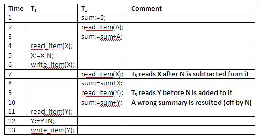
Figure 13.10
Another problem that may occur is the unrepeatable read, where a transaction T1 reads an item twice, and the item is changed by another transaction T2 between reads. Hence, T1 receives different values for its two reads of the same item.
Phantom record could occur when a transaction inserts a record into the database, which then becomes available to other transactions before completion. If the transaction that performs the insert operation fails, it appears that a record in the database disappears later.
Exercise 1
Typical problems in multi-user environment when concurrency access to data is allowed
Some problems may occur in multi-user environment when concurrency access to database is allowed. These problems may cause data stored in the multi-user DBMS to be damaged or destroyed. Four interleaved transaction schedules are given below. Identify what type of problems they have.
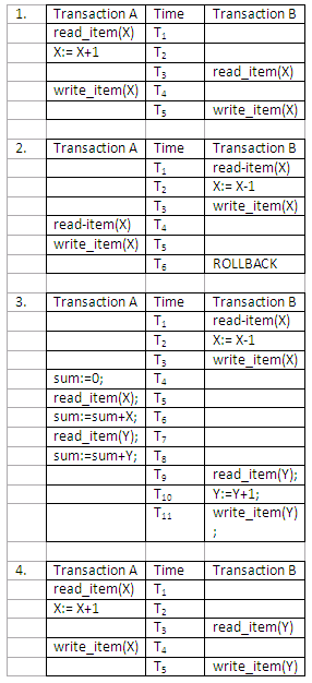
Figure 13.11
Exercise 2
Inconsistent analysis problem
Interleaved calculation of aggregates may have some aggregates on early data and some on late data if other transactions are able to update the data. This will cause incorrect summary. Consider the situation below, in which a number of account records have the following values:
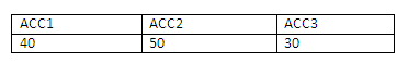
Figure 13.12
To transfer 10 from ACC3 to ACC1 while concurrently calculating the total funds in the three accounts, the following sequence of events may occur. Show the value of each data item in the last column, and discuss the reason for an incorrect summary value.
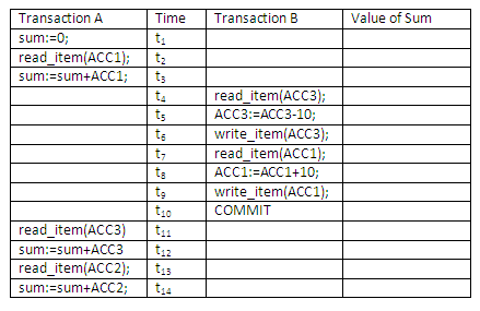
Figure 13.13
Review question 2
Whenever a transaction is submitted to a DBMS for execution, the system is responsible for making sure that either:
all the operations in the transaction are completed successfully and the effect is recorded permanently in the database; or
the transaction has no effect whatsoever on the database or on any other transactions.
The DBMS must not permit some operations of a transaction T to be applied to the database while other operations of T are not. This may happen if a transaction fails after executing some of its operations but before executing all of them.
The practical aspects of transactions are about keeping control. There are a variety of causes of transaction failure. These may include:
Concurrency control enforcement: Concurrency control method may abort the transaction, to be restarted later, because it violates serialisability (the need for transactions to be executed in an equivalent way as would have resulted if they had been executed sequentially), or because several transactions are in a state of deadlock.
Local error detected by the transaction: During transaction executions, certain conditions may occur that necessitate cancellation of the transaction (e.g. an account with insufficient funds may cause a withdrawal transaction from that account to be cancelled). This may be done by a programmed ABORT in the transaction itself.
A transaction or system error: Some operation in the transaction may cause it to fail, such as integer overflow, division by zero, erroneous parameter values or logical programming errors.
User interruption of the transaction during its execution, e.g. by issuing a control-C in a VAX/ VMS or UNIX environment.
System software errors that result in abnormal termination or destruction of the database management system.
Crashes due to hardware malfunction, resulting in loss of internal (main and cache) memory (otherwise known as system crashes).
Disk malfunctions such as read or write malfunction, or a disk read/write head crash. This may happen during a read or write operation of the transaction.
Natural physical disasters and catastrophes such as fires, earthquakes or power surges; sabotages, intentional contamination with computer viruses, or destruction of data or facilities by operators or users.
Failures of types 1 to 6 are more common than those of types 7 or 8. Whenever a failure of type 1 through 6 occurs, the system must keep sufficient information to recover from the failure. Disk failure or other catastrophic failures of 7 or 8 do not happen frequently; if they do occur, it is a major task to recover from these types of failure.
The acronym ACID indicates the properties of any well-formed transaction. Any transaction that violates these principles will cause failures of concurrency. A brief description of each property is given first, followed by detailed discussions.
Atomicity: A transaction is an atomic unit of processing; it is either performed in its entirety or not performed at all. A transaction does not partly happen.
Consistency: The database state is consistent at the end of a transaction.
Isolation: A transaction should not make its updates visible to other transactions until it is committed; this property, when enforced strictly, solves the temporary update problem and makes cascading rollbacks (see 'Atomicity' below) of transactions unnecessary.
Durability: When a transaction has made a change to the database state and the change is committed, this change is permanent and should be available to all other transactions.
Atomicity is built on the idea that you cannot split an atom. If a transaction starts, it must finish – or not happen at all. This means if it happens, it happens completely; and if it fails to complete, there is no effect on the database state.
There are a number of implications. One is that transactions should not be nested, or at least cannot be nested easily. A nested transaction is where one transaction is allowed to initiate another transaction (and so on). If one of the nested transactions fails, the impact on other transactions leads to what is known as a cascading rollback.
Transactions need to be identified. The database management system can assign a serial number of timestamp to each transaction. This identifier is required so each activity can be logged. When a transaction fails for any reason, the log is used to roll back and recover the correct state of the database on a transaction basis.
Rolling back and committing transactions
There are two ways a transaction can terminate. If it executes to completion, then the transaction is said to be committed and the database is brought to a new consistent state. Committing a transaction signals a successful end-of-transaction. It tells the transaction manager that a logical unit of work has been successfully completed, the database is (or should be) in a consistent state again, and all of the updates made by that unit of work (transaction) can now be made permanent. This point is known as a synchronisation point. It represents the boundary between two consecutive transactions and corresponds to the end of a logical unit of work.
The other way a transaction may terminate is that the transaction is aborted and the incomplete transaction is rolled back and restored to the consistent state it was in before the transaction started. A rollback signals an unsuccessful end of a transaction. It tells the transaction manager that something has gone wrong, the database might be in an inconsistent state and all of the updates made by the logical unit of work so far must be undone. A committed transaction cannot be aborted and rolled back.
Atomicity is maintained by commitment and rollback. The major SQL operations that are under explicit user control that establish such synchronisation points are COMMIT and ROLLBACK. Otherwise (default situation), an entire program is regarded as one transaction.
The database must start and finish in a consistent state. You should note that in contrast, during a transaction, there will be times where the database is inconsistent. Some part of the data will have been changed while other data has yet to be.
A correct execution of the transaction must take the database from one consistent state to another, i.e. if the database was in a consistent state at the beginning of transaction, it must be in a consistent state at the end of that transaction.
The consistency property is generally considered to be the responsibility of the programmers who write the database programs or the DBMS module that enforces integrity constraints. It is also partly the responsibility of the database management system to ensure that none of the specified constraints are violated. The implications of this are the importance of specifying the constraints and domains within the schema, and the validation of transactions as an essential part of the transactions.
A transaction should not make its update accessible to other transactions until it has terminated. This property gives the transaction a measure of relative independence and, when enforced strictly, solves the temporary update problem. In general, various levels of isolation are permitted. A transaction is said to have degree 0 isolation if it does not overwrite the dirty reads of higher-degree transactions. A degree 1 isolation transaction has no lost updates, and degree 2 isolation has no lost update and no dirty reads. Finally, degree 3 isolation (also known as true isolation) has, in addition to degree 2 properties, repeatable reads.
Isolation refers to the way in which transactions are prevented from interfering with each other. You might think that one transaction should never be interfered with by any other transactions. This is nearly like insisting on full serialisation of transactions with little or no concurrency. The issues are those of performance.
Once a transaction changes the database and the changes are committed, these changes must never be lost because of subsequent failure.
At the end of a transaction, one of two things will happen. Either the transaction has completed successfully or it has not. In the first case, for a transaction containing write_item operations, the state of the database has changed, and in any case, the system log has a record of the activities. Or, the transaction has failed in some way, in which case the database state has not changed, though it may have been necessary to use the system log to roll back and recover from any changes attempted by the transaction.
Review question 3
Discuss different types of possible transaction failures, with some examples.
Transactions cannot be nested inside one another. Why? Support your answer with an example.
This is a criterion that most concurrency control methods enforce. Informally, if the effect of running transactions in an interleaved fashion is equivalent to running the same transactions in a serial order, they are considered serialisable. We have used the word 'schedule' without a definition before in this chapter. In this section, we will first define the concept of transaction schedule, and then we characterise the types of schedules that facilitate recovery when failures occur.
When transactions are executed concurrently in an interleaved fashion, the order of execution of operations from the various transactions forms what is known as a transaction schedule (or history). A schedule S of n transactions T1, T2, … Tn is an ordering of operations of the transactions subject to the constraint that, for each transaction Ti that participates in S, the operations of Ti in S must appear in the same order in which they occur in Ti. Note, however, that operations from other transactions Tj can be interleaved with the operations of Ti in S.
Suppose that two users – airline reservation clerks – submit to the DBMS transactions T1 and T2 introduced previously at approximately the same time. If no interleaving is permitted, there are only two possible ways of ordering the operations of the two transactions for execution:
Schedule A: Execute all the operations of transaction T1 in sequence followed by all the operations of transaction T2 in sequence.
Schedule B: Execute all the operations of transaction T2 in sequence followed by all the operations of transaction T1 in sequence.
These alternatives are shown below:
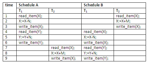
Figure 13.14
If interleaving of operations is allowed, there will be many possible orders in which the system can execute the individual operations of the transactions. Two possible schedules are shown below:
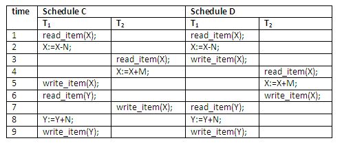
Figure 13.15
An important aspect of concurrency control, called serialisability theory, attempts to determine which schedules are 'correct' and which are not, and to develop techniques that allow only correct schedules. The next section defines serial and non-serial schedules, presents some of the serialisability theory, and discusses how it may be used in practice.
Schedules A and B are called serial schedules because the operations of each transaction are executed consecutively, without any interleaved operations from the other transaction. In a serial schedule, entire transactions are performed in serial order: T1 and then T2 or T2 and then T1 in the diagram below. Schedules C and D are called non-serial because each sequence interleaves operations from the two transactions.
Formally, a schedule S is serial if, for every transaction T participating in the schedule, all the operations of T are executed consecutively in the schedule; otherwise, the schedule is called non-serial. One reasonable assumption we can make, if we consider the transactions to be independent, is that every serial schedule is considered correct. This is so because we assume that every transaction is correct if executed on its own (by the consistency property introduced previously in this chapter) and that transactions do not depend on one another. Hence, it does not matter which transaction is executed first. As long as every transaction is executed from beginning to end without any interference from the operations of other transactions, we get a correct end result on the database. The problem with serial schedules is that they limit concurrency or interleaving of operations. In a serial schedule, if a transaction waits for an I/O operation to complete, we cannot switch the CPU processor to another transaction, thus wasting valuable CPU processing time and making serial schedules generally unacceptable.
To illustrate our discussion, consider the schedules in the diagram below, and assume that the initial values of database items are X = 90, Y = 90, and that N = 3 and M = 2. After executing transaction T1 and T2, we would expect the database values to be X = 89 and Y = 93, according to the meaning of the transactions. Sure enough, executing either of the serial schedules A or B gives the correct results. This is shown below:
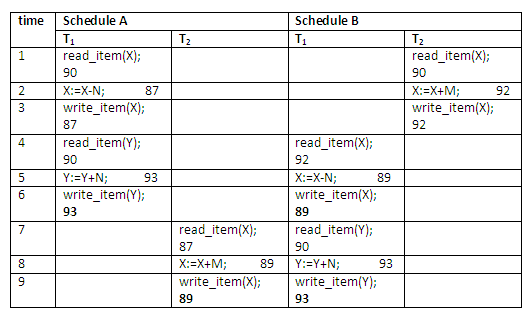
Figure 13.16
Schedules involving interleaved operations are non-serial schedules. Now consider the two non-serial schedules C and D. Schedule C gives the result X = 92 and Y = 93, in which the X value is erroneous, whereas schedule D gives the correct results. This is illustrated below:
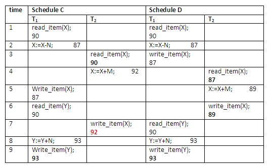
Figure 13.17
Schedule C gives an erroneous result because of the lost update problem. Transaction T2 reads the value of X before it is changed by transaction T1, so only the effect of T2 on X is reflected in the database. The effect of T1 on X is lost, overwritten by T2, leading to the incorrect result for item X.
However, some non-serial schedules do give the expected result, such as schedule D in the diagram above. We would like to determine which of the non-serial schedules always give a correct result and which may give erroneous results. The concept used to characterise schedules in this manner is that of serialisability of a schedule.
A schedule S of n transactions is a serialisable schedule if it is equivalent to some serial schedule of the same n transactions. Notice that for n transactions, there are n possible serial schedules, and many more possible non-serial schedules. We can form two disjoint groups of the non-serial schedules: those that are equivalent to one (or more) of the serial schedules, and hence are serialisable; and those that are not equivalent to any serial schedule, and hence are not serialisable.
Saying that a non-serial schedule S is serialisable is equivalent to saying that it is correct, because it is equivalent to a serial schedule, which is considered correct. For example, schedule D is a serialisable schedule, and it is a correct schedule, because schedule D gives the same results as schedules A and B, which are serial schedules. It is essential to guarantee serialisability in order to ensure database correctness.
Now the question is: when are two schedules considered 'equivalent'? There are several ways to define equivalence of schedules. The simplest, but least satisfactory, definition of schedule equivalence involves comparing the effects of the schedules on the database. Intuitively, two schedules are called result equivalent if they produce the same final state of the database. However, two schedules may accidentally provide the same final state. For example, in the figure below, schedules S1 and S2 will produce the same database state if they execute on a database with an initial value of X = 100; but for other initial values of X, the schedules are not result equivalent. Hence result equivalent is not always the safe way to define schedules equivalence.
Here are two schedules that are equivalent for the initial value of X = 100, but are not equivalent in general:
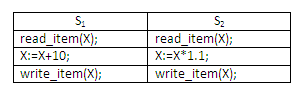
Figure 13.18
A serialisable schedule gives us the benefits of concurrent execution without giving up any correctness. In practice, however, it is quite difficult to test for the serialisability of a schedule. The interleaving of operations from concurrent operations is typically determined by the operating system scheduler. Factors such as system load, time of transaction submission, and priorities of transactions contribute to the ordering of operations in a schedule by the operating system. Hence, it is practically impossible to determine how the operations of a schedule will be interleaved beforehand to ensure serialisability. The approach taken in most practical systems is to determine methods that ensure serialisability without having to test the schedules themselves for serialisability after they are executed. One such method uses the theory of serialisability to determine protocols or sets of rules that, if followed by every individual transaction or if enforced by a DBMS concurrency control subsystem, will ensure serialisability of all schedules in which the transactions participate. Hence, in this approach we never have to concern ourselves with the schedule. In the next section of this chapter, we will discuss a number of such different concurrency control protocols that guarantee serialisability.
Exercise 3
Serial, non-serial and serialisable schedules
Given the following two transactions, and assuming that initially x = 3, and y = 2,
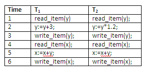
Figure 13.19
create all possible serial schedules and examine the values of x and y;
create a non-serial interleaved schedule and examine the values of x and y. Is this a serialisable schedule?
Review question 4
As a summary of schedules of transactions and serialisability of schedules, fill in the blanks in the following paragraphs:
A schedule S of n transactions T1, T2, … Tn is an ordering of the operations of the transactions. The operations in S are exactly those operations in ______ including either a ______ or ______ operation as the last operation for each transaction in the schedule. For any pair of operations from the same transaction Ti, their order of appearance in S is as their order of appearance in Ti.
In serial schedules, all operations of each transaction are executed ______ , without any operations from the other transactions. Every serial schedule is considered ______ .
A schedule S of n transactions is a fertilisable schedule if it is equivalent to some ______ of the same n transactions.
Saying that a non-serial schedule is serialisable is equivalent to saying that it is ______ , because it is equivalent to ______ .
Compare binary locks with exclusive/shared locks. Why is the latter type of locks preferable?
One of the main techniques used to control concurrency execution of transactions (that is, to provide serialisable execution of transactions) is based on the concept of locking data items. A lock is a variable associate with a data item in the database and describes the status of that data item with respect to possible operations that can be applied to the item. Generally speaking, there is one lock for each data item in the database. The overall purpose of locking is to obtain maximum concurrency and minimum delay in processing transactions.
In the next a few sections, we will discuss the nature and types of locks, present several two-phase locking protocols that use locking to guarantee serialisability of transaction schedules, and, finally, we will discuss two problems associated with the use of locks – namely deadlock and livelock – and show how these problems are handled.
The idea of locking is simple: when a transaction needs an assurance that some object, typically a database record that it is accessing in some way, will not change in some unpredictable manner while the transaction is not running on the CPU, it acquires a lock on that object. The lock prevents other transactions from accessing the object. Thus the first transaction can be sure that the object in question will remain in a stable state as long as the transaction desires.
There are several types of locks that can be used in concurrency control. Binary locks are the simplest, but are somewhat restrictive in their use.
A binary lock can have two states or values: locked and unlocked (or 1 and 0, for simplicity). A distinct lock is associated with each database item X. If the value of the lock on X is 1, item X is locked and cannot be accessed by a database operation that requests the item. If the value of the lock on X is 0, item X is unlocked, and it can be accessed when requested. We refer to the value of the lock associated with item X as LOCK(X).
Two operations, lock and unlock, must be included in the transactions when binary locking is used. A transaction requests access to an item X by issuing a lock(X) operation. If LOCK(X) = 1, the transaction is forced to wait; otherwise, the transaction sets LOCK(X) := 1 (locks the item) and allows access. When the transaction is through using the item, it issues an unlock(X) operation, which sets LOCK(X) := 0 (unlocks the item) so that X may be accessed by other transactions. Hence, a binary lock enforces mutual exclusion on the data item. The DBMS has a lock manager subsystem to keep track of and control access to locks.
When the binary locking scheme is used, every transaction must obey the following rules:
A transaction T must issue the operation lock(X) before any read_item(X) or write_item(X) operations are performed in T.
A transaction T must issue the operation unlock(X) after all read_item(X) and write_item(X) operations are completed in T.
A transaction T will not issue a lock(X) operation if it already holds the lock on item X.
A transaction T will not issue an unlock(X) operation unless it already holds the lock on item X.
These rules can be enforced by a module of the DBMS. Between the lock(X) and unlock(X) operations in a transaction T, T is said to hold the lock on item X. At most, one transaction can hold the lock on a particular item. No two transactions can access the same item concurrently.
The binary locking scheme described above is too restrictive in general, because at most one transaction can take hold on a given item. We should allow several transactions to access the same item X if they all access X for reading purposes only. However, if a transaction is to write an item X, it must have exclusive access to X. For this purpose, we can use a different type of lock called multiple-mode lock. In this scheme, there are three locking operations: read_lock(X), write_lock(X) and unlock(X). That is, a lock associated with an item X, LOCK(X), now has three possible states: 'read-locked', 'write-locked' or 'unlocked'. A read-locked item is also called share-locked, because other transactions are allowed to read access that item, whereas a write-locked item is called exclusive-locked, because a single transaction exclusively holds the lock on the item.
If a DBMS wishes to read an item, then a shared (S) lock is placed on that item. If a transaction has a shared lock on a database item, it can read the item but not update it. If a DBMS wishes to write (update) an item, then an exclusive (X) lock is placed on that item. If a transaction has an exclusive lock on an item, it can both read and update it. To prevent interference from other transactions, only one transaction can hold an exclusive lock on an item at any given time.
If a transaction A holds a shared lock on item X, then a request from another transaction B for an exclusive lock on X will cause B to go into a wait state (and B will wait until A’s lock is released). A request from transaction B for a shared lock on X will be granted (that is, B will now also hold a shared lock on X).
If transaction A holds an exclusive lock on record X, then a request from transaction B for a lock of either type on X will cause B to go into a wait state (and B will wait until A’s lock is released).
This can be summarised by means of the compatibility matrix below, that shows which type of lock requests can be granted simultaneously:
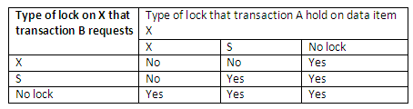
Figure 13.20
For example, when transaction A holds an exclusive (X) lock on data item X, the request from transaction B for an exclusive lock on X will not be granted. If transaction A holds a shared (S) lock on data item X, the request from transaction B for a shared lock will be granted (two transactions can read access the same item simultaneously) but not for an exclusive lock.
Transaction requests for record locks are normally implicit (at least in most modern systems). In addition, a user can specify explicit locks. When a transaction successfully retrieves a record, it automatically acquires an S lock on that record. When a transaction successfully updates a record, it automatically acquires an X lock on that record. If a transaction already holds an S lock on a record, then the update operation will promote the S lock to X level as long as T is the only transaction with an S lock on X at the time.
Exclusive and shared locks are normally held until the next synchronisation point (review the concept of synchronisation point under 'Atomicity'). However, a transaction can explicitly release locks that it holds prior to termination using the unlock command.
Using binary locks or multiple-mode locks in transactions as described earlier does not guarantee serialisability of schedules in which the transactions participate. For example, two simple transactions T1 and T2 are shown below:
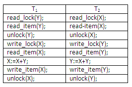
Figure 13.21
Assume, initially, that X = 20 and Y = 30; the result of serial schedule T1 followed by T2 is X = 50 and Y = 80; and the result of serial schedule T2 followed by T1 is X = 70 and Y = 50. The figure below shows an example where, although the multiple-mode locks are used, a non-serialisable schedule may still result:
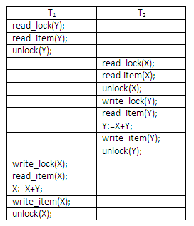
Figure 13.22
The reason this non-serialisable schedule occurs is that the items Y in T1 and X in T2 were unlocked too early. To guarantee serialisability, we must follow an additional protocol concerning the positioning of locking and unlocking operations in every transaction. The best known protocol, two-phase locking, is described below.
A transaction is said to follow the two-phase locking protocol (basic 2PL protocol) if all locking operations (read_lock, write_lock) precede the first unlock operation in the transaction. Such a transaction can be divided into two phases: an expanding (or growing) phase, during which new locks on items can be acquired but none can be released; and a shrinking phase, during which existing locks can be released but no new locks can be acquired.
Transactions T1 and T2 shown in the last section do not follow the 2PL protocol. This is because the write_lock(X) operation follows the unlock(Y) operation in T1, and similarly the write_lock(Y) operation follows the unlock(X) operation in T2. If we enforce 2PL, the transactions can be rewritten as T1’ and T2’, as shown below:
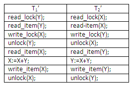
Figure 13.23
Now the schedule involving interleaved operations shown in the figure above is not permitted. This is because T1’ will issue its write_lock(X) before it unlocks Y; consequently, when T2’ issues its read_lock(X), it is forced to wait until T1’ issues its unlock(X) in the schedule.
It can be proved that, if every transaction in a schedule follows the basic 2PL, the schedule is guaranteed to be serialisable, removing the need to test for serialisability of schedules any more. The locking mechanism, by enforcing 2PL rules, also enforces serialisability.
Another problem that may be introduced by 2PL protocol is deadlock. The formal definition of deadlock will be discussed below. Here, an example is used to give you an intuitive idea about the deadlock situation. The two transactions that follow the 2PL protocol can be interleaved as shown here:
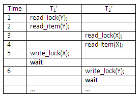
Figure 13.24
At time step 5, it is not possible for T1’ to acquire an exclusive lock on X as there is already a shared lock on X held by T2’. Therefore, T1’ has to wait. Transaction T2’ at time step 6 tries to get an exclusive lock on Y, but it is unable to as T1’ has a shared lock on Y already. T2’ is put in waiting too. Therefore, both transactions wait fruitlessly for the other to release a lock. This situation is known as a deadly embrace or deadlock. The above schedule would terminate in a deadlock.
A variation of the basic 2PL is conservative 2PL also known as static 2PL, which is a way of avoiding deadlock. The conservative 2PL requires a transaction to lock all the data items it needs in advance. If at least one of the required data items cannot be obtained then none of the items are locked. Rather, the transaction waits and then tries again to lock all the items it needs. Although conservative 2PL is a deadlock-free protocol, this solution further limits concurrency.
In practice, the most popular variation of 2PL is strict 2PL, which guarantees a strict schedule. (Strict schedules are those in which transactions can neither read nor write an item X until the last transaction that wrote X has committed or aborted). In strict 2PL, a transaction T does not release any of its locks until after it commits or aborts. Hence, no other transaction can read or write an item that is written by T unless T has committed, leading to a strict schedule for recoverability. Notice the difference between conservative and strict 2PL; the former must lock all items before it starts, whereas the latter does not unlock any of its items until after it terminates (by committing or aborting). Strict 2PL is not deadlock-free unless it is combined with conservative 2PL.
In summary, all type 2PL protocols guarantee serialisability (correctness) of a schedule but limit concurrency. The use of locks can also cause two additional problems: deadlock and livelock. Conservative 2PL is deadlock-free.
Exercise 4
Multiple-mode locking scheme and serialisability of schedules
For the example schedule shown again here below, complete the two possible serial schedules, and show the values of items X and Y in the two transactions and in the database at each time step.
Figure 13.25
Discuss why the schedule below is a non-serialisable schedule. What went wrong with the multiple-mode locking scheme used in the example schedule?
Figure 13.26
Deadlock occurs when each of two transactions is waiting for the other to release the lock on an item. A simple example was shown above, where the two transactions T1’ and T2’ are deadlocked in a partial schedule; T1’ is waiting for T2’ to release item X, while T2’ is waiting for T1’ to release item Y. Meanwhile, neither can proceed to unlock the item that the other is waiting for, and other transactions can access neither item X nor item Y. Deadlock is also possible when more than two transactions are involved.
A simple way to detect a state of deadlock is to construct a wait-for graph. One node is created in the graph for each transaction that is currently executing in the schedule. Whenever a transaction Ti is waiting to lock an item X that is currently locked by a transaction Tj, it creates a directed edge (Ti # Tj). When Tj releases the lock(s) on the items that Ti was waiting for, the directed edge is dropped from the waiting-for graph. We have a state of deadlock if and only if the wait-for graph has a cycle. Recall this partial schedule introduced previously:
Figure 13.27
The wait-for graph for the above partial schedule is shown below:
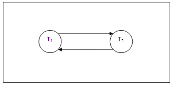
Figure 13.28
One problem with using the wait-for graph for deadlock detection is the matter of determining when the system should check for deadlock. Criteria such as the number of concurrently executing transactions or the period of time several transactions have been waiting to lock items may be used to determine that the system should check for deadlock.
When we have a state of deadlock, some of the transactions causing the deadlock must be aborted. Choosing which transaction to abort is known as victim selection. The algorithm for victim selection should generally avoid selecting transactions that have been running for a long time and that have performed many updates, and should try instead to select transactions that have not made many changes or that are involved in more than one deadlock cycle in the wait-for graph. A problem known as cyclic restart may occur, where a transaction is aborted and restarted only to be involved in another deadlock. The victim selection algorithm can use higher priorities for transactions that have been aborted multiple times, so that they are not selected as victims repeatedly.
Exercise 5
Wait-for graph
Given the graph below, identify the deadlock situations.
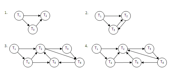
Figure 13.29
One way to prevent deadlock is to use a deadlock prevention protocol. One such deadlock prevention protocol is used in conservative 2PL. It requires that every transaction lock all the items it needs in advance; if any of the items cannot be obtained, none of the items are locked. Rather, the transaction waits and then tries again to lock all the items it needs. This solution obviously limits concurrency. A second protocol, which also limits concurrency, though to a lesser extent, involves ordering all the data items in the database and making sure that a transaction that needs several items will lock them according to that order (e.g. ascending order). For example, data items may be ordered as having rank 1, 2, 3, and so on.
A transaction T requiring data items A (with a rank of i) and B (with a rank of j, and j>i), must first request a lock for the data item with the lowest rank, namely A. When it succeeds in getting the lock for A, only then can it request a lock for data item B.
All transactions must follow such a protocol, even though within the body of the transaction the data items are not required in the same order as the ranking of the data items for lock requests. For this particular protocol to work, all locks to be applied must be binary locks (i.e. the only locks that can be applied are write locks).
A number of deadlock prevention schemes have been proposed that make a decision on whether a transaction involved in a possible deadlock situation should be blocked and made to wait, should be aborted, or should preempt and abort another transaction. These protocols use the concept of transaction timestamp TS(T), which is a unique identifier assigned to each transaction. The timestamps are ordered based on the order in which transactions are started; hence, if transaction T1 starts before transaction T2, then TS(T1) < TS(T2). Notice that the older transaction has a smaller timestamp value. This can be easily understood and remembered in the following way. For an older transaction T which is 'born' earlier, its birthday (i.e. TS(T) = 10am) is smaller than a younger transaction T’, which is 'born' at 11am (i.e. TS(T’) = 11am, and TS(T) < TS(T’) ).
Two schemes that use transaction timestamp to prevent deadlock are wait-die and wound-wait. Suppose that transaction Ti tries to lock an item X, but is not able to because X is locked by some other transaction Tj with a conflicting lock. The rules followed by these schemes are as follows:
wait-die: if TS(Ti) < TS(Tj) (Ti is older than Tj) then Ti is allowed to wait, otherwise abort Ti (Ti dies) and restart it later with the same timestamp.
wound-wait: if TS(Ti) < TS(Tj) (Ti is older than Tj) then abort Tj (Ti wound Tj) and restart it later with the same timestamp, otherwise Ti is allowed to wait.
In wait-die, an older transaction is allowed to wait on a younger transaction, whereas a younger transaction requesting an item held by an older transaction is aborted and restarted. The wound-die approach does the opposite: a younger transaction is allowed to wait on an older one, whereas an older transaction requesting an item held by a younger transaction preempts the younger transaction by aborting it. Both schemes end up aborting the younger of the two transactions that may be involved in a deadlock, and it can be shown that these two techniques are deadlock-free. The two schemes can be summarised in the following two tables. The one below is for the wait-die protocol:
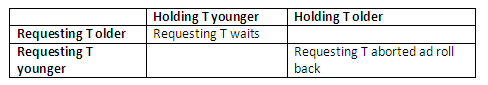
Figure 13.30
And this one below is for the wound-die protocol:
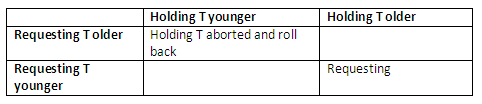
Figure 13.31
The problem with these two schemes is that they cause some transactions to be aborted and restarted even though those transactions may never actually cause a deadlock. Another problem can occur with wait-die, where the transaction Ti may be aborted and restarted several times in a row because an older transaction Tj continues to hold the data item that Ti needs.
Exercise 6
Deadlock prevention protocols
A DBMS attempts to run the following schedule. Show:
How conservative 2PL would prevent deadlock.
How ordering all data items would prevent deadlock.
How the wait-for scheme would prevent deadlock.
How the wound-wait scheme would prevent deadlock.
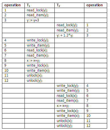
Figure 13.32
Another problem that may occur when we use locking is livelock. A transaction is in a state of livelock if it cannot proceed for an indefinite period while other transactions in the system continue normally. This may occur if the waiting scheme for locked items is unfair, giving priority to some transactions over others. The standard solution for livelock is to have a fair waiting scheme. One such scheme uses a first-come-first-serve queue; transactions are enabled to lock an item in the order in which they originally requested to lock the item. Another scheme allows some transactions to have priority over others but increases the priority of a transaction the longer it waits, until it eventually gets the highest priority and proceeds.
Review question 5
Complete the following table to describe which type of lock requests can be granted to the particular transaction.
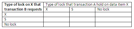
Figure 13.33
What is two-phase locking protocol? How does it guarantee serialisability?
Are the following statements true or false?
If a transaction has a shared (read) lock on a database item, it can read the item but not update it.
If a transaction has an exclusive (write) lock on a database item, it can update it but not read it.
If a transaction has an exclusive (write) lock on a database item, it can both read and update it.
If transaction A holds a shared (read) lock on a record R, another transaction B can issue a write lock on R.
Basic 2PL, conservative 2PL and strict 2PL can all guarantee serialisability of a schedule as well as prevent deadlock.
Strict 2PL guarantees strict schedules and is deadlock-free.
Conservative 2PL is deadlock-free but limits the amount of concurrency.
The wait-die and wound-wait schemes of deadlock prevention all end up aborting the younger of the two transactions that may be involved in a deadlock. They are both deadlock-free.
Complete the following tables of wait-die and wound-wait protocols for deadlock prevention.
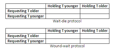
Figure 13.34
What is timestamp? Discuss how it is used in deadlock prevention protocols.
There are many new concepts in this chapter. If you want to discuss them with your colleagues or make comments about the concepts, use the online facilities.
Compare the following pairs of concepts/techniques:
Interleaved vs simultaneous concurrency
Serial vs serialisable schedule
Shared vs exclusive lock
Basic vs conservative 2PL
Wait-for vs wound-wait deadlock prevention protocol
Deadlock vs livelock
Analyse the relationships among the following terminology:
Problems of concurrency access to database (lost update, uncommitted dependency); serialisable schedule; basic 2PL; deadlock; conservative 2PL; wait-die and wound-wait
The idea of this scheme is to order the transactions based on their timestamps. (Recall the concept of timestamp.) A schedule in which the transactions participate is then serialisable, and the equivalent serial schedule has the transactions in order of their timestamp value. This is called timestamp ordering (TO). Notice the difference between this scheme and the two-phase locking. In two-phase locking, a schedule is serialisable by being equivalent to some serial schedule allowed by the locking protocols; in timestamp ordering, however, the schedule is equivalent to the particular serial order that corresponds to the order of the transaction timestamps. The algorithm must ensure that, for each item accessed by more than one transaction in the schedule, the order in which the item is accessed does not violate the serialisability of the schedule. To do this, the basic TO algorithm associates with each database item X two timestamp (TS) values:
read_TS(X): The read timestamp of item X; this is the largest timestamp among all the timestamps of transactions that have successfully read item X.
write_TS(X): The write timestamp of item X; this is the largest of all the timestamps of transactions that have successfully written item X.
Whenever some transaction T tries to issue a read_item(X) or write_item(X) operation, the basic TO algorithm compares the timestamps of T with the read and write timestamp of X to ensure that timestamp order of execution of the transactions is not violated. If the timestamp order is violated by the operation, then transaction T will violate the equivalent serial schedule, so T is aborted. Then T is resubmitted to the system as a new transaction with a new timestamp. If T is aborted and rolled back, any transaction T’ that may have used a value written by T must also be rolled back, and so on. This effect is known as cascading rollback and is one of the problems associated with the basic TO, since the schedule produced is not recoverable. The concurrency control algorithm must check whether the timestamp ordering of transactions is violated in the following two cases:
If read_TS(X)>TS(T) or if write_TS(X)>TS(T), then abort and roll back T and reject the operation. This should be done because some transaction with a timestamp greater than TS(T) – and hence after T in the timestamp ordering – has already read or written the value of item X before T had a chance to write X, thus violating the timestamp ordering.
If the condition above does not occur, then execute the write_item(X) operation of T and set write_TS(X) to TS(T).
If write_TS(X)>TS(T), then abort and roll back T and reject the operation. This should be done because some transaction with a timestamp greater than TS(T) – and hence after T in the timestamp ordering – has already written the value of item X before T had a chance to read X.
If write_TS(X) <=TS(T), then execute the read_item(X) operation of T and set read_TS(T) to the larger of TS(T) and the current read_TS(X).
Multiversion concurrency control techniques keep the old values of a data item when the item is updated. Several versions (values) of an item are maintained. When a transaction requires access to an item, an appropriate version is chosen to maintain the serialisability of the concurrently executing schedule, if possible. The idea is that some read operations that would be rejected in other techniques can still be accepted, by reading an older version of the item to maintain serialisability.
An obvious drawback of multiversion techniques is that more storage is needed to maintain multiple versions of the database items. However, older versions may have to be maintained anyway – for example, for recovery purpose. In addition, some database applications require older versions to be kept to maintain a history of the evolution of data item values. The extreme case is a temporal database, which keeps track of all changes and the items at which they occurred. In such cases, there is no additional penalty for multiversion techniques, since older versions are already maintained.
In this technique, several versions X1, X2, … Xk of each data item X are kept by the system. For each version, the value of version Xi and the following two timestamps are kept:
read_TS(Xi): The read timestamp of Xi; this is the largest of all the timestamps of transactions that have successfully read version Xi.
write_TS(Xi): The write timestamp of Xi; this is the timestamp of the transaction that wrote the value of version Xi.
Whenever a transaction T is allowed to execute a write_item(X) operation, a new version of item X, Xk+1, is created, with both the write_TS(Xk+1) and the read_TS(Xk+1) set to TS(T). Correspondingly, when a transaction T is allowed to read the value of version Xi, the value of read_TS(Xi) is set to the largest of read_TS(Xi) and TS(T).
To ensure serialisability, we use the following two rules to control the reading and writing of data items:
If transaction T issues a write_item(X) operation, and version i of X has the highest write_TS(Xi) of all versions of X which is also less than or equal to TS(T), and TS(T) < read_TS(Xi), then abort and roll back transaction T; otherwise, create a new version Xj of X with read_TS(Xj) = write_TS(Xj) = TS(T).
If transaction T issues a read_item(X) operation, and version i of X has the highest write_TS(Xi) of all versions of X which is also less than or equal to TS(T), then return the value of Xi to transaction T, and set the value of read_TS(Xj) to the largest of TS(T) and the current read_TS(Xj).
In this scheme, there are three locking modes for an item: read, write and certify. Hence, the state of an item X can be one of 'read locked', 'write locked', 'certify locked' and 'unlocked'. The idea behind the multiversion two-phase locking is to allow other transactions T’ to read an item X while a single transaction T holds a write lock X. (Compare with standard locking scheme.) This is accomplished by allowing two versions for each item X; one version must always have been written by some committed transaction. The second version X’ is created when a transaction T acquires a write lock on the item. Other transactions can continue to read the committed version X while T holds the write lock. Now transaction T can change the value of X’ as needed, without affecting the value of the committed version X. However, once T is ready to commit, it must obtain a certify lock on all items that it currently holds write locks on before it can commit. The certify lock is not compatible with read locks, so the transaction may have to delay its commit until all its write lock items are released by any reading transactions. At this point, the committed version X of the data item is set to the value of version X’, version X’ is discarded, and the certify locks are then released. The lock compatibility table for this scheme is shown below:
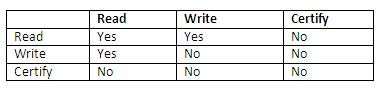
Figure 13.35
In this multiversion two-phase locking scheme, reads can proceed concurrently with a write operation – an arrangement not permitted under the standard two-phase locking schemes. The cost is that a transaction may have to delay its commit until it obtains exclusive certify locks on all items it has updated. It can be shown that this scheme avoids cascading aborts, since transactions are only allowed to read the version X that was written by committed transaction. However, deadlock may occur.
All concurrency control techniques assumed that the database was formed of a number of items. A database item could be chosen to be one of the following:
A database record.
A field value of a database record.
A disk block.
A whole file.
The whole database.
Several trade-offs must be considered in choosing the data item size. We shall discuss data item size in the context of locking, although similar arguments can be made for other concurrency control techniques.
First, the larger the data item size is, the lower the degree of concurrency permitted. For example, if the data item is a disk block, a transaction T that needs to lock a record A must lock the whole disk block X that contains A. This is because a lock is associated with the whole data item X. Now, if another transaction S wants to lock a different record B that happens to reside in the same block X in a conflicting disk mode, it is forced to wait until the first transaction releases the lock on block X. If the data item size was a single record, transaction S could proceed as it would be locking a different data item (record B).
On the other hand, the smaller the data item size is, the more items will exist in the database. Because every item is associated with a lock, the system will have a larger number of locks to be handled by the lock manger. More lock and unlock operations will be performed, causing a higher overhead. In addition, more storage space will be required for the lock table. For timestamps, storage is required for the read_TS and write_TS for each data item, and the overhead of handling a large number of items is similar to that in the case of locking.
The size of data items is often called the data item granularity. Fine granularity refers to small item size, whereas coarse granularity refers to large item size. Given the above trade-offs, the obvious question to ask is: What is the best item size? The answer is that it depends on the types of transactions involved. If a typical transaction accesses a small number of records, it is advantageous to have the data item granularity be one record. On the other hand, if a transaction typically accesses many records of the same file, it may be better to have block or file granularity so that the transaction will consider all those records as one (or a few) data items.
Most concurrency control techniques have a uniform data item size. However, some techniques have been proposed that permit variable item sizes. In these techniques, the data item size may be changed to the granularity that best suits the transactions that are currently executing on the system.
There are four suggested extension exercises for this chapter.
Interleaved concurrency
T1, T2 and T3 are defined to perform the following operations: T1: Add one to A. T2: Double A. T3: Display A on the screen and then set A to one.
Supposed the above three transactions are allowed to execute concurrently. If A has an initial value zero, how many correct results are there? Enumerate them.
Suppose the internal structure of T1, T2, and T3 is as indicated below:
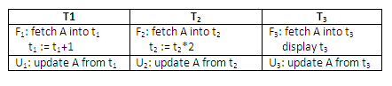
Figure 13.36
If the transactions execute without any locking, how many possible interleaved executions are there?
Deadlock
The following list represents the sequence of events in an interleaved execution of a set of transaction T1 to T12. A, B, … H are data items in the database. Assume that FETCH R acquires an S lock on R, and UPDATE R promotes that lock to X level. Assume also all locks are held until the next synchronisation point. Are there any deadlocks at time tn?
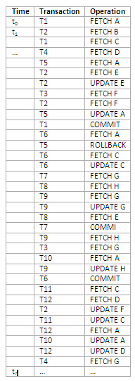
Figure 13.37
Multiversion two-phase locking
What is a certify lock? Discuss multiversion two-phase locking for concurrency control.
Granularity of data items
How does the granularity of data items affect the performance of concurrency control? What factors affect selection of granularity size for data items?