Sorting, searching and algorithm analysis

Introduction

We have learned that in order to write a computer program that performs some task, we must construct a suitable algorithm. However, the algorithm we construct is unlikely to be unique – there are likely many algorithms that perform the same task. The question then arises as to whether some of these algorithms are in any sense better than others. Algorithm analysis is the study of this question.

In this chapter we will analyze four algorithms, two for each of the following tasks:

• ordering a list of values, and
• finding the position of a value within a sorted list.

Algorithm analysis should begin with a clear statement of the task to be performed. This allows us to both check that the algorithm is correct and ensure that the algorithms we are comparing perform the same task.

Although there in general many ways that algorithms might be compared, we will focus our attention on the two that are of primary importance to many data processing algorithms:

• time complexity (how the number of steps required depends on the length of the input)
• space complexity (how the amount of extra memory or storage required depends on the length of the input)

Note

Computational complexity theory studies the inherent complexity of tasks themselves. Sometimes it is possible to prove that any algorithm that can perform a given task will require some minimum number of steps or amount of extra storage. A full introduction to computational complexity theory is outside the scope of these notes but we will mention some interesting results.

Note

The common sorting and searching algorithms are widely implemented and already available for most programming languages. You will seldom have to implement them yourself outside of the exercises in these notes. Nevertheless, understanding these algorithms is still important since you will likely be making use of them within your own programs and their space and time complexity will thus affect that of your own algorithms. You may also be required to select which sorting or searching algorithm to use which will require a good understanding of the characteristics of the algorithms available.

Sorting algorithms

Sorting a list of values is a common computational task that has been well studied. The classic description of the task is as follows:

Given a list of values and a function that compares two values, order the values in the list from smallest to largest.

The values might be integers, or strings or even other kinds of objects. We will examine two algorithms:

• Selection sort (which relies on repeatedly selecting the next smallest item), and
• Merge sort (which relies on repeatedly merging sections of the list that are already sorted)

Other well-known algorithms for sorting lists are Insertion sort, Bubble sort, Heap sort, Quicksort and Shell sort.

There are also a variety of algorithms which perform the sorting task for restricted kinds of values, for example:

• Counting sort (relies on values all belonging to a small set of items)
• Bucket sort (relies on being able to map each value to one of a small set of items)
• Radix sort (relies on values being sequences of digits)

Restricting the task enlarges the set of algorithms that can perform it and among these new algorithms may be ones that have desirable properties. For example, Radix sort uses fewer steps than any generic sorting algorithm.

Selection sort

Selection sort orders a given list by repeatedly selecting the smallest remaining element and moving it to the end of a growing sorted list.

To illustrate selection sort, let us examine how it operates on a small list of four elements:

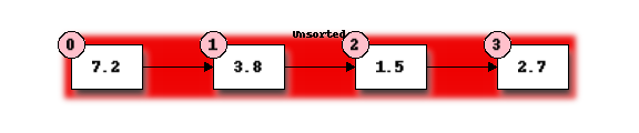
Initially the entire list is unsorted. We will use the front of the list to hold the sorted items in order to avoid using extra storage space but at the start this sorted list is empty.

First we must find the smallest element in the unsorted portion of the list. We take the first element of the unsorted list as a candidate and compare it to each of the following elements in turn, replacing our candidate with any element found to be smaller. This requires 3 comparisons and we find that element 1.5 at position 2 is smallest.

Now we will swap the first element of our unordered list with the smallest element to start our ordered list:

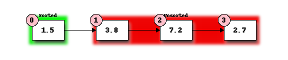
We now repeat our previous steps, determining that 2.7 is the smallest remaining element and swap it with 3.8, the first element of the current unordered section, to get:

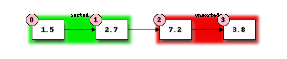
Finally, we determine that 3.8 is the smallest of the remaining unordered elements and swap it with 7.2:

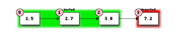
The table below shows the number of operations of each type used in sorting our example list:

Sorted List Length	Comparisons	Swaps	Assign smallest candidate
0 -> 1	3	1	3
1 -> 2	2	1	2
2 -> 3	1	1	2
Total	6	3	7

Note that the number of comparisons and the number of swaps are independent of the contents of the list (this is true for selection sort but not necessarily for other sorting algorithms) while the number of times we have to assign a new value to the smallest candidate depends on the contents of the list.

More generally, the algorithm for selection sort is as follows:

1. Divide the list to be sorted into a sorted portion at the front (initially empty) and an unsorted portion at the end (initially the whole list).
2. Find the smallest element in the unsorted list:

1. Select the first element of the unsorted list as the initial candidate.
2. Compare the candidate to each element of the unsorted list in turn, replacing the candidate with the current element if the current element is smaller.
3. Once the end of the unsorted list is reached, the candidate is the smallest element.

3. Swap the smallest element found in the previous step with the first element in the unsorted list, thus extending the sorted list by one element.
4. Repeat the steps 2 and 3 above until only one element remains in the unsorted list.

Note

The Selection sort algorithm as described here has two properties which are often desirable in sorting algorithms.

The first is that the algorithm is inplace. This means that it uses essentially no extra storage beyond that required for the input (the unsorted list in this case). A little extra storage may be used (for example, a temporary variable to hold the candidate for the smallest element). The important property is that the extra storage required should not increase as the size of the input increases.

The second is that the sorting algorithm is stable. This means that two elements which are equal, retain their initial relative ordering. This becomes important if there is additional information attached to the values being sorted (for example, if we are sorting a list of people using a comparison function that compares their dates of birth). Stable sorting algorithms ensure that sorting an already sorted list leaves the order of the list unchanged, even in the presence of elements that compare equal.

Exercise 1

Complete the following code that will perform a selection sort in Python. ”...” denotes missing code that should be filled in:

def selection_sort(items):
    """Sorts a list of items into ascending order using the
       selection sort algoright.
       """
    for step in range(len(items)):
        # Find the location of the smallest element in
        # items[step:].
        location_of_smallest = step
        for location in range(step, len(items)):
            # TODO: determine location of smallest
            ...
        # TODO: Exchange items[step] with items[location_of_smallest]
        ...

Exercise 2

Earlier in this section we counted the number of comparisons, swaps and assignments used in our example.

1. How many swaps are performed when we apply selection sort to a list of N items?
2. How many comparisons are performed when we apply selection sort to a list of N items?
   1. How many comparisons are performed when finding the smallest element when the unsorted portion of the list has M items?
   2. Sum over all the values of M encountered when sorting the list of length N to find the total number of comparisons.
3. The number of assignments (to the candidate smallest number) performed during the search for a smallest element is at most one more than the number of comparisons. Use this to find an upper limit on the total number of assignments performed while sorting a list of length N.
4. Use the results of the previous question to find an upper bound on the total number of operations (swaps, comparisons and assignments) performed? Which term in the number of operations will dominate for large lists?

Merge sort

Merge sort orders a list by repeatedly merging sorted sub-sections of the list, starting from sub-sections consisting of a single item each.

We will see shortly that merge sort requires significanly fewer operations than selection sort.

Let us start once more with our small list of four elements:

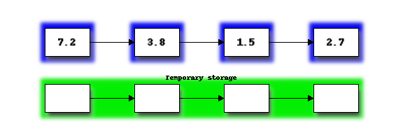
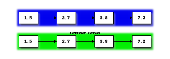
First we will merge the two sections on the left into the temporary storage. If you imagine the two sections as two sorted piles of cards, merging proceeds by repeatedly taking the smaller of the top two cards and placing it on the end of the merged list in the temporary storage. Once one of the two piles is empty, the remaining items in the other pile can just be placed on the end of the merged list:

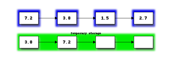
Next we copy the merged list from temporary storage, back into the portion of the list originally occupied by the merged subsections:

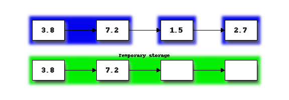
Next we repeat the procedure to merge the second pair of sorted sub-sections:

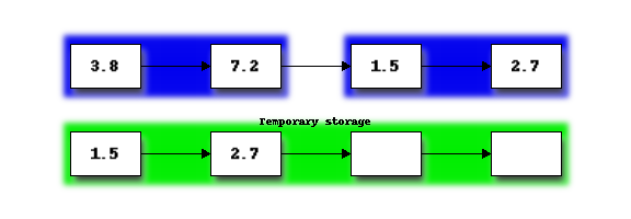
Having now reached the end of the original list, we now return to the start of list and begin merging sorted sub-sections again. We repeat this until the entire list is a single sorted sub-section. In our example, this requires just one more merge:

Here are the steps for Merge sort:

• Each element in the array is a single partition. Merge adjacent partitions to a new array, resulting in partitions of size two. Assign the new array to the original.
• Each pair of elements in the array is a single partition. Merge adjacent partitions to another new array, resulting in partitions of size four. Assign the new array to the original.
• Each group of four elements in the original array is a single partition. Merge adjacent partitions to another new array, resulting in partitions of size eight. Assign the new array to the original.
• Continue this process until the partition size is at least as large as the whole array.

Exercise 3

Write a Python function that implements merge sort. It may help to write a separate function that performs merges which you can call from within your merge sort implementation.

Python’s sorting algorithm

Python’s list objects use a sorting algorithm called Timsort invented by Tim Peters in 2002 for use in Python. Timsort is a modifed version of merge sort that uses insertion sort to arrange the list of items into conveniently mergable sections.

Note

Tim Peters is also credited as the author of The Zen of Python – an attempt to summarize the early Python community’s ethos in a short series of koans. You can read it by typing import this into the Python console.

Searching algorithms

Linear search

A linear search is the most basic kind of search method. It involves checking each element of the list in turn, until the desired element is found.

For example, suppose that we want to find the number 3.8 in the following list:

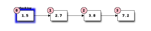
We start with the first element, and perform a comparison to see if its value is the value that we want. In this case, 1.5 is not equal to 3.8, so we move onto the next element:

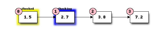
We perform another comparison, and see that 2.7 is also not equal to 3.8, so we move onto the next element:

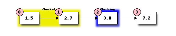
We perform another comparison and determine that we have found the correct element. Now we can end the search and return the position of the element (index 2).

We had to use a total of 3 comparisons when searching through this list of 4 elements. How many comparisons we need to perform depends on the total length of the list, but also whether the element we are looking for is near the beginning or near the end of the list. In the worst-case scenario, if our element is the last element of the list, we will have to search through the entire list to find it.

If we search the same list many times, assuming that all elements are equally likely to be searched for, we will on average have to search through half of the list each time. The cost (in comparisons) of performing a linear search thus scales linearly with the length of the list.

The advantage of linear search is that it can be performed on an unsorted list – if we are going to examine all the values in turn, their order doesn’t matter. It can be more efficient to perform a linear search than a binary search if we need to find a value once in a large unsorted list, because just sorting the list in preparation for performing a binary search could be more expensive. If, however, we need to find values in the same large list multiple times, sorting the list and using binary search becomes more worthwhile.

Exercise 4

Binary search

A binary search is a more efficient search algorithm which relies on the elements in the list being sorted. We apply the same search process to progressively smaller sub-lists of the original list, starting with the whole list and approximately halving the search area every time.

We first check the middle element in the list. If it is the value we want, we can stop. If it is higher than the value we want, we repeat the search process with the portion of the list before the middle element. If it is lower than the value we want, we repeat the search process with the portion of the list after the middle element.

For example, suppose that we want to find the value 3.8 in the following list of 7 elements:

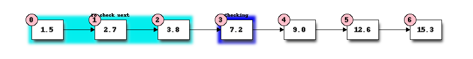
First we compare the element in the middle of the list to our value. 7.2 is bigger than 3.8, so we need to check the first half of the list next.

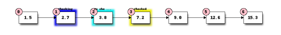
Now the first half of the list is our new list to search. We compare the element in the middle of this list to our value. 2.7 is smaller than 3.8, so we need to search the second half of this sublist next.

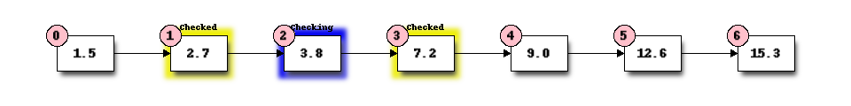
The second half of the last sub-list is just a single element, which is also the middle element. We compare this element to our value, and it is the element that we want.

We have performed 3 comparisons in total when searching this list of 7 items. The number of comparisons we need to perform scales with the size of the list, but much more slowly than for the linear search – if we are searching a list of length N, the maximum number of comparisons that we will have to perform is log₂(N).

Exercise 5

Algorithm complexity

Complexities of common operations in Python

Answers to exercises

Exercise 1

Completed selection sort implementation:

def selection_sort(items):
    """Sorts a list of items into ascending order using the
       selection sort algoright.
       """
    for step in range(len(items)):
        # Find the location of the smallest element in
        # items[step:].
        location_of_smallest = step
        for location in range(step, len(items)):
            # determine location of smallest
            if items[location] < items[location_of_smallest]:
                location_of_smallest = location
        # Exchange items[step] with items[location_of_smallest]
        temporary_item = items[step]
        items[step] = items[location_of_smallest]
        items[location_of_smallest] = temporary_item

Exercise 2

1. N - 1 swaps are performed.

2. (N - 1) * N / 2 comparisons are performed.

   1. M - 1 comparisons are performed finding the smallest element.

   2. Summing M - 1 from 2 to N gives:

      1 + 2 + 3 + ... + (N - 1)
      
      = (N - 1) * N / 2

3. At most (N - 1) * N / 2 + (N - 1) assignements are performed.

4. At most N**2 + N - 2 operations are performed. For long lists the number of operations grows as N**2.