As software engineers, we need to make informed decisions. The whole process of creating a software product, from the initial analysis of both the software's context and its requirements through to design, implementation and finally testing, requires the software development team to make decisions.
However, these decisions should not be ad hoc: software engineering, as its name implies, is currently striving to become an engineering discipline. As a field, it is working towards finding techniques and principles that will help to create both reliable and usable software, and to do so in a repeatable, predictable manner.
This underlies the need for our decisions to be informed decisions.
Now, to make informed decisions we need to have information. Sometimes the needed information is relatively easy to come by, other times not. Even when we have the information we want we can often be unsure of its value. To help solve these problems we can use methods from the field of statistics, an area of scientific enquiry meant for information gathering and analysis. Statistics is the mathematical field that concerns itself with decision making, and excels itself with the measurement and quantification of uncertainty.
Statistics is the science of decision making when dealing with uncertainty.
Statistics is useful when the information we need is not straight forward to obtain. For a simple example, consider software meant to replace an existing product, with the goal of reducing the number of errors being performed, both by the software itself, and by the end users of the software. Statistics supplies us with tools for the measurement of the error rates associated with both the original and new systems, as well as for the analysis of the final results. It supplies a firm, mathematical basis for deciding whether the new software reduces the amount of errors, or for concluding that any changes between the systems are artefacts of our testing, with the actual error rates between the two systems being identical.
Although statistics is fundamentally a mathematical discipline, its use does not necessarily demand any deep mathematical knowledge. These notes do not concern themselves with the mathematical underpinnings of the field. You will not need to be capable of doing more than follow a handful of simple formula, each of which use nothing more complicated than simple arithmetic.
Statistics is a large field, and these notes are nowhere near long enough to do anything more then briefly introduce the field, giving a hint as to the depth and flavour of statistical analysis. For further information, the interested reader is pointed to one of the following introductory books on the subject:
L. Underhill & D. Bradfield (1996). IntroStat. Juta & Co, Ltd: Epping
R. R. Sokal (1995). Biometry: the Principles and Practice of Statistics in Biological Research. Freeman: New York
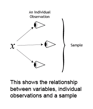
Statistics is a tool for dealing with information. We gain information by making observations, by taking measurements. These 'things' that we measure are called variables. Examples of variables are error rates or response times in user testing, number of errors per lines of code for software metrics, number of simultaneous connections that a database can carry, etc.
An individual observation is the actual measurement (or observation) of a variable. For example, if 'error rate' is the variable that we are measuring, the actual rate that each person achieves is an individual observation of that variable. All of the individual observations taken together make up the sample of observations (also known as the sample). In other words, the sample of observations is the set of values obtained when measuring the variable of interest.

There is a special set of observations that needs to be mentioned: the population. The population is the set of all individual observations about which inferences are to be made. It is the largest sample of observations that could ever be taken. How does this differ from a sample of observations? A sample of observations is defined as being a set of individual observations. The population is the set of all individual observations. This means that a sample of observations can be a subset of the population. This distinction is necessary because of a problematic fact that occurs in research: it is often extremely difficult, if not impossible, to obtain all of the individual observations of a variable. Consider this extended example:
If Microsoft wanted to perform usability testing on their next release of Word, they would first need to identify the variables that they wish to measure, for example the error rates, or perhaps the average number of mouse clicks to perform an operation.
Next, Microsoft needs to obtain individual observations of these variables. The collection of these observations is their sample.
Ideally, Microsoft would want to obtain individual observations of each variable from each and every potential user. However, considering how many people use Word, this is not something easily done. Microsoft would need to satisfy itself with testing only a small portion of Word's potential users.
Because they are not testing all of their potential users, their sample of observations is going to be smaller than it ideally should be: instead of testing everyone, they are only testing some of them. Hence they would only have a subset of the total number of individual observations, a sample of observations from the population of observations. Naturally, it is the population that one would want to make inferences about, and one of the goals of statistical analysis is to have our inferences which are based on a sample of observations remain valid once applied to the population.
There are two general methods of determining information about the world:
we can either observe the world, noting the relationships that occur between the variables we are interested in
or we can try to manipulate the variables, and then determine what changes these manipulations have caused
The first method is a 'weaker' form of information gathering than the second, although it is easier to perform and also convenient for the exploratory analysis of data. This method is concerned with correlations and regressions, asking questions such as:
Is there a relationship of some form between the variables we are interested in, and how strong is this relationship (correlations)?
If we have values for certain variables, can we predict the values of other variables, and with what accuracy can this be done (this is known as regression)?
Although extremely useful, correlations (and regression analysis) have one flaw that often means that we need to make use of techniques from method two: they fail to make statements concerning the causality between two variables. Consider:
It can be shown that there is a relationship between users that feel 'stupid' concerning their computer skills, and software that is difficult to use. In other words, there is a correlation between perceived levels of one's own 'stupidity' and how 'usable' a software product is. Now, from knowing only that a relationship exists, can one show, whether the system is difficult to use because the users are lacking in computer skills, or that the users perceive themselves as lacking these skills because the system is difficult to use? This is an illustration of the problem associated with correlations and regression analyses: they do not offer a sense of direction in terms of cause and effect. They only state that there is a relationship between variables, and not what the relationship is.
The techniques of method two are those concerned with controlled experiments. These experiments control all the important factors concerning the variables that we are interested in, and then manipulate some of these factors in order to determine how they relate to other variables.
Note that experiments differ in two important ways to methods in group one above:
Experiments are active: they manipulate variables taking part in the experiment
Experiments determine directionality: they can answer questions of cause and effect
There are two types of variables involved in experimental research: variables that we manipulate, and variables we only observe, and that depend in some way on the manipulated variables. The first group of variables are known as independent variables, meaning that they do not rely on any other variables present in the experiment. The latter set of variables are called the dependant variables, since they depend on the independent variables.
One of the simplest experimental designs consists of obtaining two samples of the variables that we are interested in. One can see the need for having two samples by thinking about the properties of a controlled experiment: experiments want to manipulate the independent variables so as to determine the change that doing so brings about in the dependant variables. This can only be done if we have a 'baseline': we need to know what the individual observations for the dependent variables would be if the independent variables were not manipulated. Otherwise how can we tell how they have changed?
The sample taken where the independent variables are not manipulated is known as the control group. The sample obtained by manipulating the independent variables is known as the experimental group.
These two samples are then statistically compared to each other to determine if there is a difference that occurs between the dependent variables of the two experiments. Without the presence of the control group we could not begin thinking of answering questions of cause and effect.
Note that for a two-sample experiment to work correctly, the only changes between the control and the experimental samples should occur to the independent variables, otherwise other changes, not being properly noted by the experimenters, might influence the dependent variables and corrupt the results.
Not all experiments consist of only two sample groups, there being some that deal with three or more samples. However, performing and analysing experiments of this kind is beyond the scope of these notes.
When dealing with experiments we often need to know how much confidence we can place in their results. This implies that we need to know how well our sample represents the population. In other words, we need to know the degree to which our experiment is externally valid.
For example, imagine that we have been hired to replace a company's existing software with a product that needs to reduce error rates by 15 percent. On testing our new software, we discover that our product reduces error rates by 20 percent. We need to know if our tests hold for all possible individual observations of the error rates, i.e. for the population of error rates.
It could happen that once we install the software we see only a small reduction in the error rate, or perhaps even an increase. With money at stake, what assurances do we have that the results of our testing will hold up in the work environment?
To gain a degree of certainty in our results, statistical analyses are performed on the samples of our experiment in order to determine a confidence level that can be attached to the result. A confidence level gives us a probability that our results are not within some certain range. For example, a confidence level for the above example will give a probability that the new error rate is below 15 percent. The smaller the confidence level, the more likely it is that our experiment has valid results.
Often we know what confidence level we are attempting to achieve, and we can then design our experiments in attempt to achieve these confidence levels. This 'target' for our confidence levels we call our significance levels. Note that the only difference between the confidence and significance level is that the significance level is target created before the statistical analysis begins, while the confidence level is the true, calculated level.
If the confidence levels reach the target set by our significance levels, then we say that our results are significant.
Perhaps the simplest 'statistic' that is calculated from the sample is the mean, which, as its name implies, is the average of the sample:

Here N is the number of observations (i.e. the size of the sample), and Xi is an individual observation from the sample. The mean is usually represented by the symbol on the left hand side of the equation, pronounced X-bar:
We would hope that if the sample was large enough, and constructed randomly enough, that the sample mean would approximate the population mean. Because we usually do not know the population mean, we use confidence levels to give us assurances that the sample mean lies within some distance from the true population mean.
The mean is one of the basic units that more complicated statistical analyses are built upon, and will be used later when performing t-tests.
The end goal of performing statistical research is to learn about the population after only seeing the sample. One of the assumptions made to simplify this process concerns how the individual observations are 'spread' through the population. This is known as a distribution.
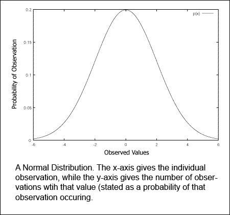
A normal distribution
For example, many populations will tend to have a normal distribution. A normal distribution occurs when most of the individual observations lie around the population's mean. Fewer observations occur the more their values diverge from the mean.
If we can assume that the population we are studying has a normal distribution, then we can make useful estimates of certain probabilities based on this. For example, it is less likely that the sample mean would lie far away from the true population mean than it is for it to lie close to the mean.
Even though normal distributions each have the same general shape, they can differ from each other in how quickly their values 'taper off' as you move away from the mean. This 'spread' is measured by a value known as the variance, usually represented as s2. The smaller the variance, the narrower the distribution. The larger the variance, the broader. The variance needs to be taken into account when considering how close the sample mean could lie to the population mean. Consider two populations P1 and P2, each, respectively, with a sample S1 and S2. Also assume that P1 and P2 have the same mean, as do S1 and S2, and that P2 has a greater variance than P1. This would allow the sample mean of S2 to lie farther away from the true population mean.
Associated with the variance is the standard deviation, usually denoted as s. Like the variance, the standard deviation is also a measure of a normal distribution's spread, although in a more readable form: the units associated with the s are the same units associated with the individual observations. The standard deviation defines a range around the distribution's mean (between -1 and +1 standard deviations around the mean) in which approximately 68.2% of the individual observations lie. The region of the distribution laying between +3 and -3 standard deviations of from the mean contain approximately 99.8% of all the individual observations.
Just as we cannot directly calculate the population mean, only the sample mean, we cannot directly calculate either the population variance or the population standard deviation.
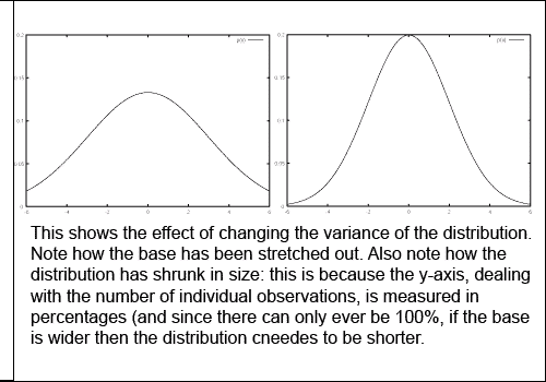
The effect of variance
Along with the mean, the variance and the standard deviations form the basic building blocks to statistical analysis. We have already seen how to calculate the mean, and now we will have a look at calculating both the variance and the standard deviation.
The first two steps are to calculate the mean, as we have done above, and then to calculate the sums of squares of differences from the mean:

The squared value is a measure of the distance of Xi (where Xi is an individual observation) to the mean, and SS is the sum of these distances. There is an alternative 'shortcut' formula for calculating the same value, but which requires less work. It is:

Note that N is, once again, the sample size.
We have the following sample of observations
3, 6, 3, 8, 9, 23First we calculate the mean:

Now we will use the 'shortcut' formula to calculate SS. First we calculate the squared values of the sample:

Next we sum these values:

And then square the mean and divide by N:

And now we perform the final subtraction:
SS = 728 - 12.5185 = 715.4815And you can check this value by calculating SS using the other formula.
Now that we have SS defined, we can easily define the both the variance and the standard deviation. The variance is simply:

If we consider the first equation given for SS, we can see that the variance is almost the average of the squared differences of the individual observations and the mean. If one thinks of the definition of the mean, the variance should have been divided by N instead of N - 1 for it to be a mean. In fact, the definition of variance as it stands is expected to be that average, but corrected for an effect called bias. Bias effects the ability of an average sample value to recreate the average population value.
The standard deviation is easily defined from the variance:

Using the same sample as the SS sample above, we can calculate the variance as:

And the standard deviation is:

For all experiments there are two possible ways of interpreting the results. For example, imagine our experiments have shown that our new application takes a user 5% less time than previous tests. This could be interpreted in two ways: this improvement in time could be due to our application, or this improvement in time could be due to sampling error. Every controlled experiment could have these two possible outcomes, and they are given names:
H0: Our manipulations of the independent variable has had no effect. Any changes observed in the dependent variables are due to incorrect sampling of the population.
H1: Our manipulations of the independent variable has had a significant effect on the dependent variables.
We call H0 the null hypothesis. Our goal when performing the experimental research is to show that the null hypothesis is false, and we do so for some significance level.
Many statistical tests make assumptions about the data upon which they are used. It is important to make sure these assumptions are met in order for the test to produce an accurate and reliable result. A common assumption is whether or not data is normally distributed, so it is important for us to be able to test for normality before further analysis so that we use the correct tests for our data thereafter.
There are several different statistical tests that allow us to see if our sample is normally distributed. The Shapiro-Wilk test is one such test which works well even for small sample sizes, and has been shown to perform better than other tests for normality.
The Shapiro-Wilk test uses the null hypothesis principle to test if a sample comes from a normally distributed population.
H0: The data in the sample are taken from a normal distribution (the sample is normally distributed)
H1: The data in the sample are not taken from a normal distribution (the sample is not normally distributed).
In order to use the test, we first rearrange the data in ascending order. Then we calculate SS as follows:

Next, we calculate b:

where m = n/2 if n is even and m = (n-1)/2 otherwise, and the values for ai are taken from Table 1 of the Shapiro-Wilk tables, based on n, the size of our sample.
Now we calculate W, the test statistic: W = b2/SS.
Finally, we look up the corresponding p value for the value of W that we have calculated in Table 2 of the Shapiro-Wilk tables. If p < 0.05, we reject the null hypothesis - our data is not normally distributed. If p > 0.05, then the null hypothesis is not rejected, and we can assume that our sample is normally distributed.
This section shows how we can compare two samples to each other in order to determine if there is a significant difference between them (in other words, if these two samples are from two different populations).
This comparison is done between the averages of the samples, and takes the variance into account. Note that one of the assumptions made when using the t test is that the populations the samples are from are normally distributed. If they are not normally distributed, then the t tests will give incorrect results.
t test comparison
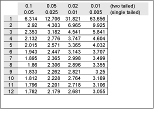
The t test involves calculating a value, let us call it t, and then comparing this value to a critical t value. This critical value is calculated from a normal distribution, and takes into account your required significance levels. The critical t value is usually looked up from a table, such as this one
The t test begins by calculating a combined variance for the two samples, using the following equation:

The value N1 + N2 - 2 is called the degrees of freedom (actually, this is a combined degrees of freedom, where the degrees of freedom for a single sample is merely N - 1).
Next, we calculate the standard error of difference:

Finally, we calculate t:

To complete the test requires a table lookup. Note that the table has values for both a 'two-tailed' and a 'single-tailed' significance level. This is named after where in the normal distribution we are looking for the null hypothesis to lie: the null hypothesis can only be true around the population mean of distribution. If we seek to reject the null hypothesis, we need our sample mean (in this case, the combined means) to lie far enough away from the population mean in order for us to consider the null hypothesis as false. This means that we reject the null hypothesis if our sample mean lies at the tails of the distribution. If we are not concerned in the 'direction' that the sample differs (i.e. whether it is greater or smaller than the population mean), we use the two-tailed test. Otherwise we use the single-tailed test. We look up a value for the degrees of freedom and required level of significance. If our calculated t value exceeds the t value from the tables, then we may reject the null hypothesis.
Note that if we are using a two tailed test, we must ignore the sign of our calculated t value (i.e. if our calculated t value is negative, ignore the negative sign).
Suppose that we have two samples
S1: 3, 6, 3, 8, 9, 23
S2: 8, 11, 12, 4, 15, 19
First we calculate SS1 and SS2. SS1 has been previously calculated, and is 715.4815.
Similarly, SS2 is 908.9583 (the reader can confirm this using one of the equations given for calculating SS). Next, we calculate the combined variance:

We now calculate t:

Now we use the table above to look up a two tailed critical t value (two tailed because we are looking to reject a null hypothesis that could occur at either end of the distribution). Our degrees of difference is 10, and our chosen significance level is 0.05 (i.e. there is a 5% chance of the null hypothesis being true). Looking in the table, we see that our critical t is 2.228.
Ignoring signs, we see that our calculated t is less than our critical t, and so we cannot reject the null hypothesis, and must conclude that the two samples came from the same population.
Sometimes it will be necessary to compare the mean of a sample to some value. For instance, perhaps we would like to know if the number of user errors is less than a certain upper limit. Although this comparison can be easily made (you just compare the mean to this value), we would still like to know the confidence levels associated with this. We can use the t test to do this.
In the case where we only have one sample, the t test is still calculated in a similar manner to the above, with the only exception being that the formulas are now simply changed to reflect the fact that only one sample is being tests.
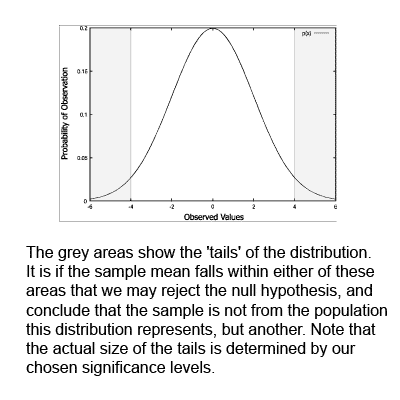
The tails of a distribution
This method of comparison is performed by constructing an interval from the two extreme positions in which the population mean may lie. This interval is called a confidence interval. This interval should either lie completely above or below the stated limiting value. For example, if we need the number of user errors to be below 10 per day, then this whole interval must lay below 10 per day. On the other hand, if we wanted to show that the error rates where now above 10 per day, then the whole interval would have to lie above this value.
The simplified version of the t test is as follows:


Note that the standard error of differences is now called the standard error of the mean. Now, instead of calculating a value for t, we calculate the interval:

Where c is a value looked up in the above t test table. It is looked up for a given significance level and degrees of freedom (which in this case is N - 1). In other words, we can choose the maximum significance level, and compute the corresponding confidence level from that. Note that for any given degree of freedom, smaller significance levels give larger values of c, forcing our confidence intervals to become larger and larger.
For this test we use the one-tailed values. This is because we are interested in our sample mean being either larger or smaller than a given value, but not both.
For the sample
3, 6, 3, 8, 9, 23determine if the mean of the population that this was drawn from is below 10.
We first begin by calculating SS, as has been done previously. The relevant information is repeated here:

SS = 715.4815
Note that the sample mean is below the value 10. Calculating the confidence intervals (note that from the formula for determining the interval we can see that this interval always lays around the mean) for a given significance level, and seeing that this interval is below the value 10, will allow us to conclude that the population mean is below the value 10 at the given significance levels.
Now we calculate the variance, which is:

We now calculate:

Let us choose a significance level of 0.05. We need to remember to use a single-tailed value. Our c is 1.943.
Next we calculate the intervals:

So our interval lies from -0.8222 to 18.1554. Comparing this with 10, we see that the interval does not lie completely below this interval: 10 lies within the interval. Hence, at a significance level of 0.05, we must conclude that the population mean is not below the value 10.
The Mann-Whitney's U test is basically a non-parametric version of the t test. Just like the t test, this test compares two samples to each other in order to determine if there is a significant difference between them. However, this test should be used when your data is not normally distributed.
Assume we have collected the following data from two groups (group 1 and group 2):
Sample 1: 3, 4, 2, 6, 2, 5
Sample 2: 9, 7, 5, 10, 6, 8
The first step is to assign a rank to every observation starting with rank 1 for the smallest value. If two or more values are tied, they are given a rank equal to the midpoint between them. The ranks for the values are shown in parentheses below:
Sample 1: 3(3), 4(4), 2(1.5), 6(7.5), 2(1.5), 5(5.5)
Sample 2: 9(11), 7(9), 5(5.5), 10(12), 6(7.5), 8(10)
Notice that 2 is the lowest value. Ordinarily, it would be assigned a rank of 1. However, because more than one observation has this value, we have to resolve the tie by assigning a rank value equal to the midpoint of the contended ranks ((1+2)/2 = 1.5). The ranks for other tied values are calculated in the same way.
Now that we have ranked each observation, we sum the ranks for each sample.
R1 = 3 + 4 + 1.5 + 7.5 + 1.5 + 5.5 = 23
R2 = 11 + 9 + 5.5 + 12 + 7.5 + 10 = 55
Next, we calculate Ui for each sample using the following equations:

where ni is the sample size for the sample i, and Ri is the rank sum for sample i that we just calculated.
So U1 = 34 and U2 = 2.
Now, we arrive at U itself, which is just the smaller of the two U values above: U = min(U1, U2). So U = 2.
Finally, we have to look up the critical value for U based on the sizes of our two samples in the Mann-Whitney tables. This reveals that the critical U value for sample sizes both equal to 6 is 5. Our U value is smaller than this, so we reject the null hypothesis. There is a significant difference between our two samples.