Figure 2.1
Table of contents
At the end of this chapter you should be able to:
Describe the structure of the Relational model, and explain why it provides a simple but well-founded approach to the storage and manipulation of data.
Explain basic concepts of the Relational model, such as primary and foreign keys, domains, null values, and entity and referential integrity.
Be able to discuss in terms of business applications, the value of the above concepts in helping to preserve the integrity of data across a range of applications running on a corporate database system.
Explain the operators used in Relational Algebra.
Use Relational Algebra to express queries on Relational databases.
In parallel with this chapter, you should read Chapter 3 and Chapter 4 of Thomas Connolly and Carolyn Begg, "Database Systems A Practical Approach to Design, Implementation, and Management", (5th edn.).
The aim of this chapter is to explain in detail the ideas underlying the Relational model of database systems. This model, developed through the '70s and '80s, has grown to be by far the most commonly used approach for the storing and manipulation of data. Currently all of the major suppliers of database systems, such as Oracle, IBM with DB2, Sybase, Informix, etc, base their products on the Relational model. Two of the key reasons for this are as follows.
Firstly, there is a widely understood set of concepts concerning what constitutes a Relational database system. Though some of the details of how these ideas should be implemented continue to vary between different database systems, there is sufficient consensus concerning what a Relational database should provide that a significant skill base has developed in the design and implementation of Relational systems. This means that organisations employing Relational technology are able to draw on this skill-base, as well as on the considerable literature and consultancy know-how available in Relational systems development.
The second reason for the widespread adoption of the Relational model is robustness. The core technology of most major Relational products has been tried and tested over the last 12 or so years. It is a major commitment for an organisation to entrust the integrity, availability and security of its data to software. The fact that Relational systems have proved themselves to be reliable and secure over a significant period of time reduces the risk an organisation faces in committing what is often its most valuable asset, its data, to a specific software environment.
Relational Algebra is a procedural language which is a part of the Relational model. It was originally developed by Dr E. F. Codd as a means of accessing data in Relational databases. It is independent of any specific Relational database product or vendor, and is therefore useful as an unbiased measure of the power of Relational languages. We shall see in a later chapter the further value of Relational Algebra, in helping gain an understanding of how transactions are processed internally within the database system.
The Relational model underpins most of the major database systems in commercial use today. As such, an understanding of the ideas described in this chapter is fundamental to these systems. Most of the remaining chapters of the module place a strong emphasis on the Relational approach, and even in those that examine research issues that use a different approach, such as the chapter on Object databases, an understanding of the Relational approach is required in order to draw comparisons and comprehend what is different about the new approach described. The material on Relational Algebra provides a vendor-independent and standard approach to the manipulation of Relational data. This information will have particular value when we move on to learn the Structured Query Language (SQL), and also assist the understanding of how database systems can alter the ways queries were originally specified to reduce their execution time, a topic covered partially in the chapter called Database Administration and Tuning.
Much of the theory underpinning the Relational model of data is derived from mathematical set theory. The seminal work on the theory of Relational database systems was developed by Dr E. F. Codd, (Codd 1971). The theoretical development of the model has continued to this day, but many of the core principles were described in the papers of Codd and Date in the '70s and '80s.
The application of set theory to database systems provides a robust foundation to both the structural and data-manipulation aspects of the Relational model. The relations, or tables, of Relational databases, are based on the concepts of mathematical sets. Sets in mathematics contain members, and these correspond to the rows in a relational table. The members of a set are unique, i.e. duplicates are not allowed. Also the members of a set are not considered to have any order; therefore, in Relational theory, the rows of a relation or table cannot be assumed to be stored in any specific order (note that some database systems allow this restriction to be overridden at the physical level, as in some situations, for example to improve the performance response of the database, it can be desirable to ensure the ordering of records in physical storage).
We saw in the previous chapter, that the Relational model uses one simple data structure, the table, to represent information. The rows in tables correspond to specific instances of records, for example, a row of a customer table contains information about a particular customer. Columns in a table contain information about a particular aspect of a record, for example, a column in a customer record might contain a customer’s contact telephone number.
Much of the power and robustness of the Relational approach derives from the use of simple tabular structures to represent data. To illustrate this, consider the information that might typically be contained in part of the data dictionary of a database. In a data dictionary, we will store the details of logical table structures, the physical allocations of disk space to tables, security information, etc. This data dictionary information will be stored in tables, in just the same way that, for example, customer and other information relevant to the end users of the system will be stored.
This consistency of data representation means that the same approach for data querying and manipulation can be applied throughout the system.
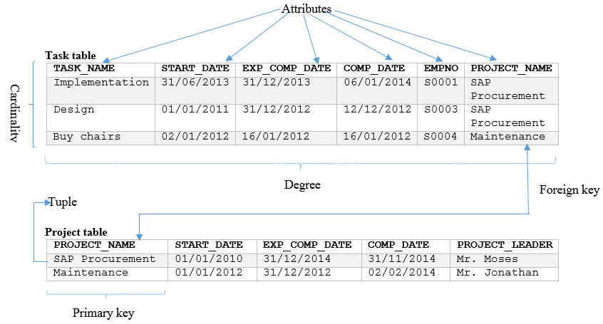
A relation is a table with columns and tuples. A database can contain as many tables as the designer wants. Each table is an implementation of a real-world entity. For example, the university keeps information about students. A student is represented as an entity during database design stage. When the design is implemented, a student is represented as a table. You will learn about database design is later modules.
An attribute is a named column in the table. A table can contain as many attributes as the designer wants. Entities identified during database design may contain attributes/characteristics that describe the entity. For example, a student has a student identification number and a name. Student identification and name will be implemented as columns in the student table.
The domain is the allowable values for a column in the table. For example, a name of a student can be made of a maximum of 30 lower and upper case characters. Any combination of lower and upper case characters less or equal to 30 is the domain for the name column.
A tuple is the row of the table. Each tuple represents an instance of an entity. For example, a student table can contain a row holding information about Moses. Moses is an instance of the student entity.
The degree of a relation/table is the number of columns it contains.
The cardinality of a relation/table is the number of rows it contains.
In the previous chapter, we described the use of primary keys to identify each of the rows of a table. The essential point to bear in mind when choosing a primary key is that it must be guaranteed to be unique for each different row of the table, and so the question you should always ask yourself is whether there is any possibility that there could be duplicate values of the primary key under consideration. If there is no natural candidate from the data items in the table that may be used as the primary key, there is usually the option of using a system-generated primary key. This will usually take the form of an ascending sequence of numbers, a new number being allocated to each new instance of a record as it is created. System-generated primary keys, such as this, are known as surrogate keys. A drawback to the use of surrogate keys is that the unique number generated by the system has no other meaning within the application, other than serving as a unique identifier for a row in a table. Whenever the option exists therefore, it is better to choose a primary key from the available data items in the rows of a table, rather than opting for an automatically generated surrogate key.
Primary keys may consist of a single column, or a combination of columns. An example of a single table column would be the use of a unique employee number in a table containing information about employees.
As an example of using two columns to form a primary key, imagine a table in which we wish to store details of project tasks. Typical data items we might store in the columns of such a task table might be: the name of the task, date the task was started, expected completion date, actual completion date, and the employee number of the person responsible for ensuring the completion of the task. There is a convenient, shorthand representation for the description of a table as given above: we write the name of the table, followed by the name of the columns of the table in brackets, each column being separated by a comma. For example:
TASK (TASK_NAME, START_DATE, EXPECTED_COMP_DATE, COMP_DATE, EMPNO)
We shall use this convention for expressing the details of the columns of a table in examples in this and later chapters. Choosing a primary key for the task table is straightforward while we can assume that task names are unique. If that is the case, then we may simply use task name as the primary key. However, if we decide to store in the task table, the details of tasks for a number of different projects, it is less likely that we can still be sure that task names will be unique. For example, supposing we are storing the details of two projects, the first to buy a new database system, and the second to move a business to new premises. For each of these projects, we might have a task called 'Evaluate alternatives'. If we wish to store the details of both of these tasks in the same task table, we can now no longer use TASK_NAME as a unique primary key, as it is duplicated across these two tasks.
As a solution to this problem, we can combine the TASK_NAME column with something further to add the additional context required to provide a unique identifier for each task. In this case, the most sensible choice is the project name. So we will use the combination of the PROJECT_NAME and TASK_NAME data items in our task table in order to identify uniquely each of the tasks in the table. The task table becomes:
TASK (PROJECT_NAME, TASK_NAME, START_DATE, EXPECTED_COMP_DATE, COMP_DATE, EMPNO)
We may, on occasions, choose to employ more than two columns as a primary key in a table, though where possible this should be avoided as it is both unwieldy to describe, and leads to relatively complicated expressions when it comes to querying or updating data in the database. Notice also that we might have used a system-generated surrogate key as the solution to the problem of providing a primary key for tasks, but the combination of PROJECT_NAME and TASK_NAME is a much more meaningful key to users of the application, and is therefore to be preferred.
Very often we wish to relate information stored in different tables. For example, we may wish to link together the tasks stored in the task table described above, with the details of the projects to which those tasks are related. The simplicity by which this is achieved within the Relational model, is one of the model's major strengths. Suppose the Task and Project tables contain the following attributes:
TASKS (TASK_NAME, START_DATE, EXP_COMP_DATE, COMP_DATE, EMPNO)
PROJECT (PROJECT_NAME, START_DATE, EXP_COMP_DATE, COMP_DATE, PROJECT_LEADER)
We assume that TASK_NAME is an appropriate primary key for the TASK table, and PROJECT_NAME is an appropriate primary key for the PROJECT table.
In order to relate a record of a task in a task table to a record of a corresponding project in a project table, we use a concept called a foreign key. A foreign key is simply a piece of data that allows us to link two tables together. In the case of the projects and tasks example, we will assume that each project is associated with a number of tasks. To form the link between the two tables, we place the primary key of the PROJECT table into the TASK table. The task table then becomes:
TASK (TASK_NAME, START_DATE, EXP_COMP_DATE, COMP_DATE, EMPNO, PROJECT_NAME)
Through the use of PROJECT_NAME as a foreign key, we are now able to see, for any given task, the project to which it belongs. Specifically, the tasks associated with a particular project can now be identified simply by virtue of the fact that they contain that project’s name as a data item as one of their attributes. Thus, all tasks associated with a research project called GENOME RESEARCH, will contain the value of GENOME RESEARCH in their PROJECT_NAME attribute.
The beauty of this approach is that we are forming the link using a data item. We are still able to maintain the tabular structure of the data in the database, but can relate that data in whatever ways we choose. Prior to the development of Relational systems, and still in many non-Relational systems today, rather than using data items in this way to form the link between different entity types within a database, special link items are used, which have to be created, altered and removed. These activities are in addition to the natural insertions, updates and deletions of the data itself. By using a uniform representation of data both for the data values themselves, and the links between different entity types, we achieve uniformity of expression of queries and updates on the data.
The need to link entity types in this way is a requirement of all, other than the most trivial of, database applications. That it occurs so commonly, allied with the simplicity of the mechanism for achieving it in Relational systems, has been a major factor in the widespread adoption of Relational databases.
Below is the summary of the concepts we have covered so far:
Figure 2.1
Integrity constraints are restrictions that affect all the instances of the database.
There is a standard means of representing information that is not currently known or unavailable within Relational database systems. We say that a column for which the value is not currently known, or for which a value is not applicable, is null. Null values have attracted a large amount of research within the database community, and indeed for the developers and users of database systems they can be an important consideration in the design and use of database applications (as we shall see in the chapters on the SQL language).
An important point to grasp about null values is that they are a very specific way of representing the fact that the data item in question literally is not currently set to any value at all. Prior to the use of null values, and still in some systems today, if it is desired to represent the fact that a data item is not currently set to some value, an alternative value such as 0, or a blank space, will be given to that data item. This is poor practice, as of course 0, or a blank space, are perfectly legitimate values in their own right. Use of null values overcomes this problem, in that null is a value whose meaning is simply that there is no value currently allocated to the data item in question.
There are a number of situations in which the use of null values is appropriate. In general we use it to indicate that a data item currently has no value allocated to it. Examples of when this might happen are:
When the value of the data item is not yet known.
When the value for that data item is yet to be entered into the system.
When it is not appropriate that this particular instance of the data item is given a value.
An example of this last situation might be where we are recording the details of employees in a table, including their salary and commission. We would store the salaries of employees in one table column, and the details of commission in another. Supposing that only certain employees, for example sales staff, are paid commission. This would mean that all employees who are not sales staff would have the value of their commission column set to null, indicating that they are not paid commission. The use of null in this situation enables us to represent the fact that some commissions are not set to any specific value, because it is not appropriate to pay commission to these staff.
Another result of this characteristic of null values is that where two data items both contain null, if you compare them with one another in a query language, the system will not find them equal. Again, the logic behind this is that the fact that each data item is null does not mean they are equal, it simply means that they contain no value at all.
As briefly discussed in Chapter 1, in Relational databases, we usually use each table to store the details of particular entity types in a system. Therefore, we may have a table for Customers, Orders, etc. We have also seen the importance of primary keys in enabling us to distinguish between different instances of entities that are stored in the different rows of a table.
Consider for the moment the possibility of having null values in primary keys. What would be the consequences for the system?
Null values denote the fact that the data item is not currently set to any real value. Imagine, however, that two rows in a table are the same, apart from the fact that part of their primary keys are set to null. An attempt to test whether these two entity instances are the same will find them not equal, but is this really the case? What is really going on here is that the two entity instances are the same, other than the fact that a part of their primary keys are as yet unknown. Therefore, the occurrence of nulls in primary keys would stop us being able to compare entity instances. For this reason, the column or columns used to form a primary key are not allowed to contain null values. This rule is known as the Entity Integrity Rule, and is a part of the Relational theory that underpins the Relational model of data. The rule does not ensure that primary keys will be unique, but by not allowing null values to be included in primary keys, it does avoid a major source of confusion and failure of primary keys.
If a foreign key is present in a given table, it must either match some candidate value in the home table or be set to null. For example, in our project and task example above, every value of PROJECT_NAME in the task table must exist as a value in the PROJECT_NAME column of the project table, or else it must be set to null.
These are additional rules specified by the users or database administrators of a database, which define or constrain some aspect of the enterprise. For example, a database administrator can contain the PROJECT_NAME column to have a maximum of 30 characters for each value inserted.
Restrict (also known as 'select') is used on a single relation, producing a new relation by excluding (restricting) tuples in the original relation from the new relation if they do not satisfy a condition; thus only the tuples required are selected.
This operation has the effect of choosing certain tuples (rows) from the table, as illustrated in the diagram below.
The use of the term 'select' here is quite specific as an operation in the Relational Algebra. Note that in the database query language SQL, all queries are phrased using the term 'select'. The Relational Algebra 'select' means 'extract tuples which meet specific criteria'. The SQL 'select' is a command that means 'produce a table from existing relations using Relational Algebra operations'.
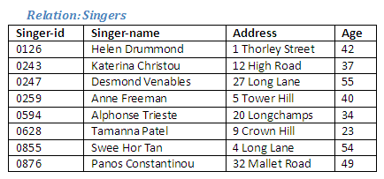
Figure 2.2
Using the Relational Algebra, extract from the relation Singers those individuals who are over 40 years of age, and create a new relation called Mature-Singers.
Relational Algebra operation: Restrict from Singers where age > 40 giving Mature-Singers
We can see which tuples are chosen from the relation Singers, and these are identified below:
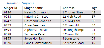
Figure 2.3
The new relation, Mature-Singers, contains only those tuples for singers aged over 40 extracted from the relation Singers. These were shown highlighted in the relation above.
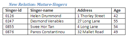
Figure 2.4
Note that Anne Freeman (age 40) is not shown. The query explicitly stated those over 40, and therefore anyone aged exactly 40 is excluded.
If we wanted to include singers aged 40 and above, we could use either of the following operations which would have the same effect.
Either:
Relational Algebra operation: Restrict from Singers where age >= 40 giving Mature-Singers2
or
Relational Algebra operation: Restrict from Singers where age > 39 giving Mature-Singers2
The result of either of these operations would be as shown below:
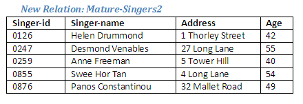
Figure 2.5
Project is used on a single relation, and produces a new relation that includes only those attributes requested from the original relation. This operation has the effect of choosing columns from the table, with duplicate entries removed.
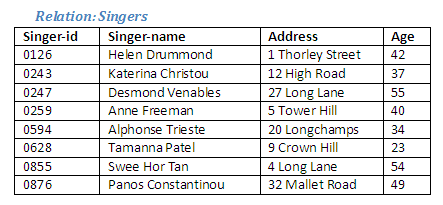
Figure 2.6
The task here is to extract the names of the singers, without their ages or any other information as shown in the diagram below. Note that if there were two singers with the same name, they would be distinguished from one another in the relation Singers by having different singer-id numbers. If only the names are extracted, the information that there are singers with the same name will not be preserved in the new relation, as only one copy of the name would appear.
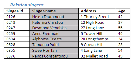
Figure 2.7
The column for the attribute singer-names is shown highlighted in the relation above.
The following Relational Algebra operation creates a new relation with singer-name as the only attribute.
Relational Algebra operation: Project Singer-name over Singers giving Singer-names
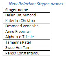
Figure 2.8
Union (also called 'append') forms a new relation of all tuples from two or more existing relations, with any duplicate tuples deleted. The participating relations must be union compatible.
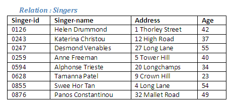
Figure 2.9
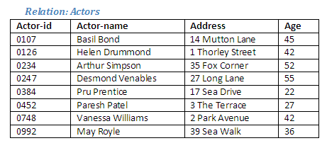
Figure 2.10
It can be seen that the relations Singers and Actors have the same number of attributes, and these attributes are of the same data types (the identification numbers are numeric, the names are character fields, the address field is alphanumeric, and the ages are integer values). This means that the two relations are union compatible. Note that it is not important whether the relations have the same number of tuples.
The two relations Singers and Actors will be combined in order to produce a new relation Performers, which will include details of all singers and all actors. An individual who is a singer as well as an actor need only appear once in the new relation. The Relational Algebra operation union (or append) will be used in order to generate this new relation.
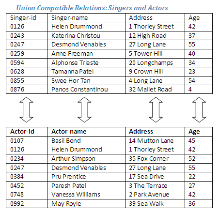
Figure 2.11
The union operation will unite these two union-compatible relations to form a new relation containing details of all singers and actors.
Relational Algebra operation: Union Singers and Actors giving Performers
We could also express this activity in the following way:
Relational Algebra operation: Union Actors and Singers giving Performers
These two operations would generate the same result; the order in which the participating relations are given is unimportant. When an operation has this property it is known as commutative - other examples of this include addition and multiplication in arithmetic. Note that this does not apply to all Relational Algebra operations.
The new relation Performers contains one tuple for every tuple that was in the relation Singers or the relation Actors; if a tuple appeared in both Singers and Actors, it will appear only once in the new relation Performers. This is why there is only one tuple in the relation Performers for each of the individuals who are both actors and singers (Helen Drummond and Desmond Venables), as they appear in both the original relations.
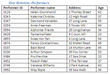
Figure 2.12
Intersection creates a new relation containing tuples that are common to both the existing relations. The participating relations must be union compatible.
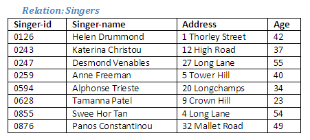
Figure 2.13
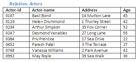
Figure 2.14
As before, it can be seen that the relations Singers and Actors are union compatible as they have the same number of attributes, and corresponding attributes are of the same data type.
We can see that there are some tuples that are common to both relations, as illustrated in the diagram below. It is these tuples that will form the new relation as a result of the intersection operation.
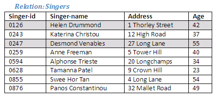
Figure 2.15
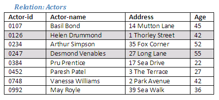
Figure 2.16
The Relational Algebra operation intersection will extract the tuples common to both relations, and use these tuples to create a new relation.
Relational Algebra operation: Actors Intersection Singers giving Actor-Singers
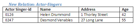
Figure 2.17
The intersection of Actors and Singers produces a new relation containing only those tuples that occur in both of the original relations. If there are no tuples that are common to both relations, the result of the intersection will be an empty relation (i.e. there will be no tuples in the new relation).
Note that an empty relation is not the same as an error; it simply means that there are no tuples in the relation. An error would occur if the two relations were found not to be union compatible.
Difference (sometimes referred to as 'remove') forms a new relation by excluding tuples from one relation that occur in another. The resulting relation contains tuples that were present in the first relation only, but not those that occur in both the first and the second relations, or those that occur in the second relation alone. This operation can be regarded as 'subtracting' tuples in one relation from another relation. The participating relations must be union compatible.
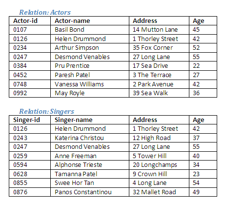
Figure 2.18
If we want to find out which actors are not also singers, the following Relational Algebra operation will achieve this:
Relational Algebra operation: Actors difference Singers giving Only-Actors
The result of this operation is to remove from the relation Actors those tuples that also occur in the relation Singers. In effect, we are removing the tuples in the intersection of Actors and Singers in order to create a new relation that contains only actors. The diagram below shows which tuples are in both relations.
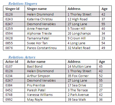
Figure 2.19
The new relation Only-Actors contains tuples from the relation Actors only if they were not also present in the relation Singers.
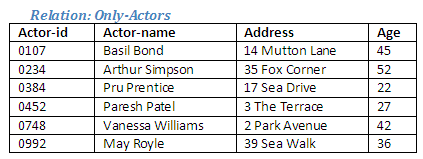
Figure 2.20
It can be seen that this operation produces a new relation Only-Actors containing all tuples in the relation Actors except those that also occur in the relation Singers.
If it is necessary to find out which singers are not also actors, this can be done by the relational operation 'remove Actors from Singers', or 'Singers difference Actors'. This operation would not produce the same result as 'Actors difference Singers' because the relational operation difference is not commutative (the participating relations cannot be expressed in reverse order and achieve the same result).
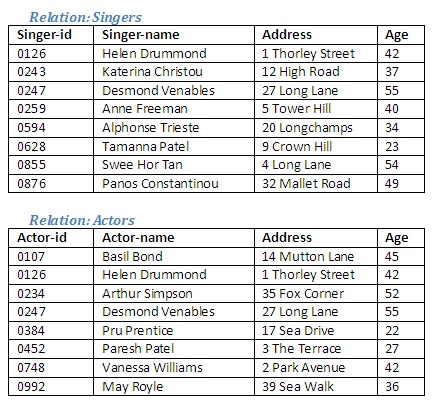
Figure 2.21
Relational Algebra operation: Singers difference Actors giving Only-Singers
The effect of this operation is to remove from the relation Singers those tuples that are also present in the relation Actors. The intersection of the two relations is removed from the relation Singers to create a new relation containing tuples of those who are only singers. The intersection of the relations Singers and Actors is, of course, the same as before.
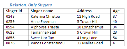
Figure 2.22
This operation produces a new relation Only-Singers containing all tuples in the relation Singers except those that also occur in the relation Actors. The tuples that are removed from one relation when the difference between two relations is generated are those that are in the intersection of the two relations.
If a relation called Relation-A has a certain number of tuples (call this number N), this can be represented as NA (meaning the number of tuples in Relation-A). Similarly, Relation-B may have a different number of tuples (call this number M), which can be shown as MB (meaning the number of tuples in Relation-B).
The resulting relation from the operation 'Relation-A Cartesian product Relation-B' forms a new relation containing NA * MB tuples (meaning the number of tuples in Relation-A times the number of tuples in Relation-B). Each tuple in the new relation created as a result of this operation will consist of each tuple from Relation-A paired with each tuple from Relation-B, which includes all possible combinations.
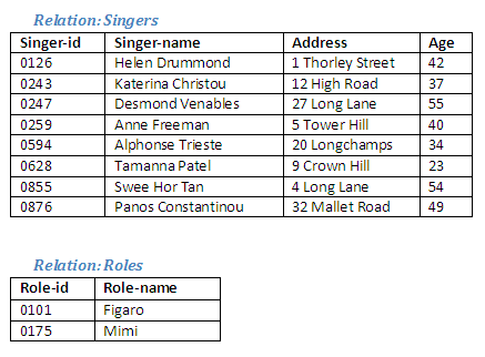
Figure 2.23
In order to create a new relation which pairs each singer with each role, we need to use the relational operation Cartesian product.
Relational Algebra operation: Singers Cartesian product Roles giving Singers-Roles
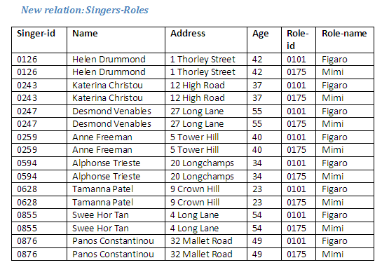
Figure 2.24
The result of Singers Cartesian product Roles gives a new relation Singers-Roles, showing each tuple from one relation with each tuple of the other, producing the tuples in the new relation. Each singer is associated with all roles; this produces a relation with 16 tuples, as there were 8 tuples in the relation Singers, and 2 tuples in the relation Roles.
What do you think would be the result of the following?
Relational Algebra operation: Singers Cartesian product Singers giving Singers-Extra
Relational Algebra operation: Actors Cartesian product Roles giving Actors-Roles
The Relational Algebra operation 'Relation-A divide by Relation-B giving Relation-C' requires that the attributes of Relation-B must be a subset of those of Relation-A. The relations do not need to be union compatible, but they must have some attributes in common. The attributes of the result, Relation-C, will also be a subset of those of Relation-A. Division is the inverse of Cartesian product; it is sometimes easier to think of the operation as similar to division in simple algebra and arithmetic.
In arithmetic:
If, for example:
Value-A = 2
Value-B = 3
Value-C = 6
then: Value-C is the result of Value-A times Value-B (i.e. 6 = 2 * 3) and: Value-C divided by Value-A gives Value-B as a result(i.e. 6/2 = 3) and: Value-C divided by Value-B gives Value-A as a result (i.e. 6/3 = 2)
In Relational Algebra:
If:
Relation-A = Singers
Relation-B = Roles
Relation-C = Singers-Roles
then: Relation-C is the result of Relation-A Cartesian product Relation-B and: Relation-C divided by Relation-A gives Relation-B as a result
and: Relation-C divided by Relation-B gives Relation-A as a result.
If we start with two relations, Singers and Roles, we can create a new relation Singers-Roles by performing the Cartesian product of Singers and Roles. This new relation shows every role in turn with every singer.
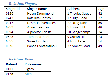
Figure 2.25
The new relation Singers-Roles has a special relationship with the relations Singers and Roles from which it was created, as will be demonstrated below.
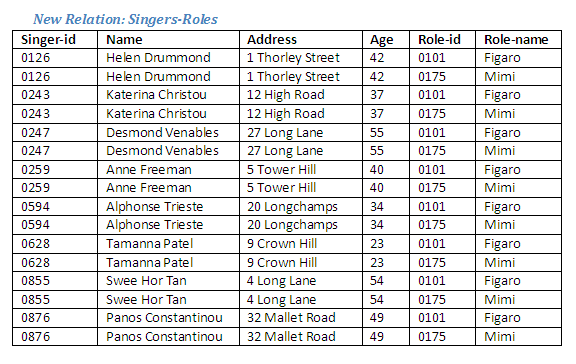
Figure 2.26
We can see that the attributes of the relation Singers are a subset of the attributes of the relation Singers-Roles. Similarly, the attributes of the relation Roles are also a subset (although a different subset) of the relation Singers-Roles.
If we now divide the relation Singers-Roles by the relation Roles, the resulting relation will be the same as the relation Singers.
Relational Algebra operation: Singers-Roles divide by Roles giving Our-Singers
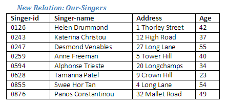
Figure 2.27
Similarly, if we divide the relation Singers-Roles by the relation Singers, the relation that results from this will be the same as the original Roles relation.
Relational Algebra operation: Singers-Roles divide by Singers giving Our-Roles
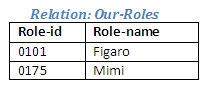
Figure 2.28
Note that there are only two tuples in this relation, although the attributes role-id and role-name appeared eight times in the relation Singer-Roles, as each role was associated with each singer in turn.
In the case where not all tuples in one relation have corresponding tuples in the 'dividing' relation, the resulting relation will only contain those tuples which are represented in both the 'dividing' and 'divided' relations. In such a case it would not be possible to recreate the 'divided' relation from a Cartesian product of the 'dividing' and resulting relations. The next example demonstrates this.
Consider the relation Recordings shown below, which holds details of the songs recorded by each of the singers.
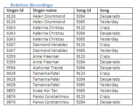
Figure 2.29
Three individuals, Chris, Mel and Sam, have each created two new relations listing their favourite songs and their favourite singers. The use of the division operation will enable Chris, Mel and Sam to find out which singers have recorded their favourite songs, and also which songs their favourite singers have recorded.
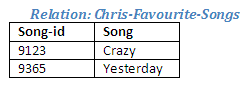
Figure 2.30
The table above contains Chris's favourite songs. In order to find out which singers have made a recording of these songs, we need to divide this relation into the Recordings relation. The result of this Relational Algebra operation is a new relation containing the details of singers who have recorded all of Chris's favourite songs. Singers who have recorded some, but not all, of Chris's favourite songs are not included.
Relational Algebra operation: Recordings divide by Chris-Favourite-Songs giving Chris-Singers-Songs
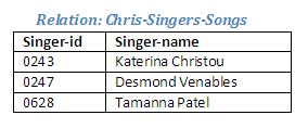
Figure 2.31
Note that the singers in this relation are not the same as those in the relation Chris-Favourite-Singers. The reason for this is that Chris's favourite singers have not all recorded Chris's favourite songs.
The next relation shows Chris's favourite singers. Chris wants to know which songs these singers have recorded. If we divide the Recordings relation by this relation, we will get a new relation that contains the songs that all these singers have recorded; songs that have been recorded by some, but not all, of the singers will not be included in the new relation.
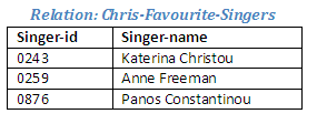
Figure 2.32
The singers in this relation are not the same as those who sing Chris's favourite songs. The reason for this is that not all of Chris's favourite singers have recorded these songs.
In order to discover the songs recorded by Chris's favourite singer, we need to divide the relation Recordings by Chris-Favourite-Songs.
Relational Algebra operation: Recordings divide by Chris-Favourite-Songs giving Chris-Songs-by-Singers
The new relation created by this operation will provide us with the information about which of Chris's favourite singers has recorded all of Chris's chosen songs. Any singer who has recorded some, but not all, of Chris's favourite songs will be excluded from this new relation.
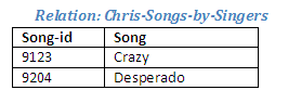
Figure 2.33
We can see that the relation created to identify the songs recorded by Chris's favourite singers is not the same as Chris's list of favourite songs, because these singers have not all recorded the songs listed as Chris's favourites.
In this example, we have been able to generate two new relations by dividing into the Recordings relation. These two new relations do not correspond with the other two relations that were divided into the relation Recordings, because there is no direct match. This means that we could not recreate the Recordings relation by performing a Cartesian product operation on the two relations containing Chris's favourite songs and singers.
In the next example, we will identify the songs recorded by Mel's favourite singers, and which singers have recorded Mel's favourite songs. In common with Chris's choice, we will find that the singers and the songs do not match as not all singers have recorded all songs. If all singers had recorded all songs, the relation Recordings would be the result of Singers Cartesian product Songs, but this is not the case.
Mel's favourite songs include all those that have been recorded, but not all singers have recorded all songs. Mel wants to find out who has recorded these songs, but the result will only include those singers who have recorded all the songs.
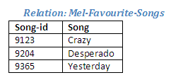
Figure 2.34
There are no other songs that have been recorded from the list available; Mel has indicated that all of these are favourites.
The relational operation below will produce a new relation, Mel-Singers-Songs, which will contain details of those singers who have recorded all of Mel's favourite songs.
Relational Algebra operation: Recordings divide by Mel-Favourite-Songs giving Mel-Singers-Songs
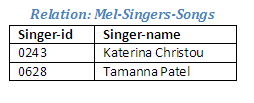
Figure 2.35
We can see from this relation, and the one below, that none of Mel's favourite singers has recorded all of the songs selected as Mel's favourites.
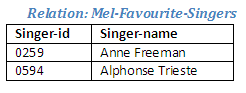
Figure 2.36
We can use the relation Mel-Favourite-Singers to find out which songs have been recorded by both these performers.
Relational Algebra operation: Recordings divide by Mel-Favourite-Singers giving Mel-Songs-by-Singers
There is only one song that has been recorded by the singers Mel has chosen, as shown in the relation below.
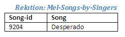
Figure 2.37
We can now turn our attention to Sam's selection of songs and singers. It happens that Sam's favourite song is the same one that Mel's favourite singers have recorded.

Figure 2.38
If we now perform the reverse query to find out who has recorded this song, we find that there are more singers who have recorded this song than the two who were Mel's favourites. The reason for this difference is that Mel's query was to find out which song had been recorded by particular singers. This contrasts with Sam's search for any singer who has recorded this song.
Relational Algebra operation: Recordings divide by Sam-Favourite-Songs giving Sam-Singer-Songs
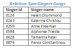
Figure 2.39
Here we can see that Mel's favourite singers include the performers who have recorded Sam's favourite song, but there are many other singers who have also made a recording of the same song. Indeed, there are only two singers who have not recorded this song (Desmond Venables and Swee Hor Tan). This could be considered unfortunate for Sam, as these are the only two singers named as Sam's favourites.
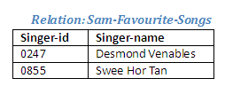
Figure 2.40
We know that the only two singers who have not recorded Sam's favourite song are in fact Sam's favourite singers. It is now our task to discover which songs these two singers have recorded.
Relation Algebra operation: Recordings divide by Sam-Favourite-Singers giving Sam-Songs-by-Singers
This operation creates a new relation that reveals the identity of the song that has been recorded by all of Sam's favourite singers.
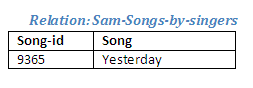
Figure 2.41
There is only one song that these two singers have recorded. Indeed, Swee Hor Tan has only recorded this song, and therefore whatever other songs had been recorded by Desmond Venables, this song is the only one that fulfils the criteria of being recorded by both these performers.
Join forms a new relation with all tuples from two relations that meet a condition. The relations might happen to be union compatible, but they do not have to be.
The following two relations have a conceptual link, as the stationery orders have been made by some of the singers. Invoices can now be generated for each singer who placed an order. (Note that we would not wish to use Cartesian product here, as not all singers have placed an order, and not all orders are the same.)
The relation Orders identifies the stationery items (from the Stationery relation) that have been requested, and shows which customer ordered each item (here the customer-id matches the singer-id).
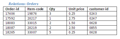
Figure 2.42
The Singers relation contains the names and addresses of all singers (who are the customers), allowing invoices to be prepared by matching the customers who have placed orders with individuals in the Singers relation.
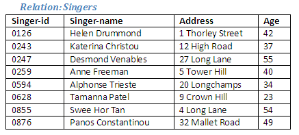
Figure 2.43
Relational Algebra operation: Join Singers to Orders where Singers Singer-id = Orders Customer-id giving Invoices
The relation Singers is joined to the relation Orders where the attribute Singer-id in Singers has the same value as the attribute Customer-id in Orders, to form a new relation Invoices.
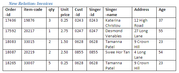
Figure 2.44
The attribute which links together the two relations (the identification number) occurs in both original relations, and thus is found twice in the resulting new relation; the additional occurrence can be removed by means of a project operation. A version of the join operation, in which such a project is assumed to occur automatically, is known as a natural join.
The types of join operation that we have used so far, and that are in fact by far most commonly in use, are called equi-joins. This is because the two attributes to be compared in the process of evaluating the join operation are compared for equality with one another. It is possible, however, to have variations on the join operation using operators other than equality. Therefore it is possible to have a GREATER THAN (>) JOIN, or a LESS THAN (<) JOIN.
It would have been possible to create the relation Invoices by producing the Cartesian product of Singers and Orders, and then selecting only those tuples where the Singer-id attribute from Singers and the Customer-id attribute from Orders has the same value. The join operation enables two relations which are not union compatible to be linked together to form a new relation without generating a Cartesian product, and then extracting only those tuples which are required.
Let X be the set of student tuples for students studying databases, and Y the set of students who started university in 1995. Using this information, what would be the result of:
X union Y
X intersect Y
X difference Y
Describe, using examples, the characteristics of an equi-join and a natural join.
Consider the following relation A with attributes X and Y,
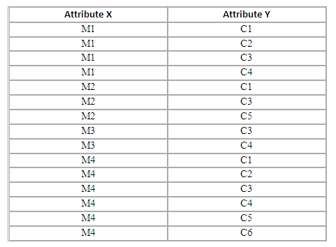
Figure 2.45
and a relation B with only one attribute (attribute Y). Assume that attribute Y of relation A and the attribute of relation B are defined on a common domain. What would be the result of A divided by B if:
B = Attribute Y C1
B = Attribute Y C2 C3
Briefly describe the theoretical foundations of Relational database systems.
Describe what is meant if a data item contains the value 'null'.
Why is it necessary sometimes to have a primary key that consists of more than one attribute?
What happens if you test two attributes, each of which contains the value null, to find out if they are equal?
What is the Entity Integrity Rule?
How are tables linked together in the Relational model?
What is Relational Algebra?
Explain the concept of union compatibility.
Describe the operation of the Relational Algebra operators RESTRICT, PROJECT, JOIN and DIVIDE.
Now that you have been introduced to the structure of the Relational model, and having seen important mechanisms such as primary keys, domains, foreign keys and the use of null values, discuss what you feel at this point to be the strengths and weaknesses of the model. Bear in mind that, although the Relational Algebra is a part of the Relational model, it is not generally the language used for manipulating data in commercial database products. That language is SQL, which will be covered in subsequent chapters.
Consider the operations of Relational Algebra. Why do you think Relational Algebra is not used as a general approach to querying and manipulating data in Relational databases? Given that it is not used as such, what value can you see in the availability of a language for manipulating data which is not specific to any one developer of database systems?
As we have seen, the Relational Algebra is a useful, vendor-independent, standard mechanism for discussing the manipulation of data. We have seen, however, that the Relational Algebra is rather procedural and manipulates data one step at a time. Another vendor-independent means of manipulating data has been developed, known as Relational Calculus. For students interested in investigating the language aspect of the Relational model further, it would be valuable to compare what we have seen so far of the Relational Algebra, with the approach used in Relational Calculus. Indeed, it possible to map expressions between the Algebra and the Calculus, and it has also been shown that it is possible to convert any expression in one language to an equivalent expression in the other. In this sense, the Algebra and Calculus are formally equivalent.