Figure 3.1
Table of contents
At the end of this chapter you should be able to:
Write SQL queries to examine the data in the rows and columns of relational tables.
Use string, arithmetic, date and aggregate functions to perform various calculations or alter the format of the data to be displayed.
Sort the results of queries into ascending or descending order.
Understand the significance of NULL entries and be able to write queries that deal with them.
In parallel with this chapter, you should read Chapter 5 of Thomas Connolly and Carolyn Begg, "Database Systems A Practical Approach to Design, Implementation, and Management", (5th edn.).
This chapter introduces the fundamentals of the Structured Query Language, SQL, which is a worldwide standard language for the querying and manipulation of Relational databases. This chapter covers the basic concepts of the language, and sufficient information for you to write simple but powerful queries. The further chapters on the SQL language will build on this knowledge, covering more complex aspects of the query language and introducing statements for adding, changing and removing data and the tables used to contain data. The material you will cover in the SQL chapters provides you with a truly transferable skill, as the language constructs you will learn will work in virtually all cases, unchanged, across a wide range of Relational systems.
This unit presents the basics of the SQL language, and together with the succeeding units on SQL, provides a detailed introduction to the SQL language. The unit relates to the information covered on Relational Algebra, in that it provides a practical example of how the operations of the algebra can be made available within a higher level, non-procedural language. This chapter also closely relates to the material we will later cover briefly on query optimisation in a chapter called Database Administration and Tuning, as it provides the basic concepts needed to understand the syntax of the language, which is the information on which the query optimisation software operates.
There are a number of SQL implementations out there, including Microsoft Access (part of the Office suite), Microsoft SQL server and Oracle. There are also some open-source ones such as MySQL. You should make sure you have an SQL implementation installed for this chapter. Consult the course website for more information about the recommended and/or compatible SQL implementations. Although SQL commands in these notes are written in generic terms, you should be mindful that SQL implementations are different and sometimes what is given here may not work, or will work with slight modification. You should consult the documentation of your software on the particular command should what is given here not work with your SQL implementation.
SQL is a language that has been developed specifically for querying and manipulating data in database systems. Its facilities reflect this fact; for example, it is very good for querying and altering sets of database records collectively in one statement (this is known as set-level processing). On the other hand, it lacks some features commonly found in general programming languages, such as LOOP and IF…THEN…ELSE statements.
SQL stands for Structured Query Language, and indeed it does have a structure, and is good for writing queries. However, it is structured rather differently to most traditional programming languages, and it can be used to update information as well as for writing queries.
SQL, as supported in most database systems, is provided via a command-line interface or some sort of graphical interface that allows for the text-based entry of SQL statements. For example, the following SQL statement is a query that will list the names of departments from a database table (also known as a relation) called DEPT:
SELECT DNAME FROM DEPT;
SQL language consists of three major components:
DDL (data definition language): Used to define the way in which data is stored.
DML (data manipulation language): Allows retrieval, insertion of data, etc. (This is sometimes called the 'query' language.)
DCL (data control language): Used to control access to the data. For example, granting access to a user to insert data in a particular table.
The query language (DML) is very flexible in that it can be used to express quite complicated queries, sometimes very concisely.
One initial problem that people just starting to learn the language encounter is that it can sometimes be difficult to tell how hard a query will be to express in SQL from its natural language specification. That is, some queries that sound as though they will be hard to code in SQL from their description in a natural language such as English, turn out to be very straightforward. However, some simple-sounding queries turn out to be surprisingly difficult.
As you work through the SQL chapters in this module, you will build up experience and knowledge of the kinds of queries that are straightforward to write in SQL.
The data manipulation language (DML) of SQL allows the retrieval, insertion, updating and removal of rows stored in relational tables. As mentioned above, numbers of rows can be altered in any one statement, and so DML is a very powerful tool.
The data definition language (DDL) is used to create, change the structure of or remove whole tables and other relational structures. So whereas you would use the INSERT statement of the DML to insert new rows into an existing table, you would use the DDL CREATE TABLE statement to establish a new table in the first place.
The data control language (DCL) defines activities that are not in the categories of those for the DDL and DML, such as granting privileges to users, and defining when proposed changes to a databases should be irrevocably made.
Throughout this and the succeeding chapters on SQL, we are going to use a standard pair of tables and set of data on which to write SQL statements. This standard data set comprises the tables EMP and DEPT. The structure of each is first described, and then the example records for each are presented.
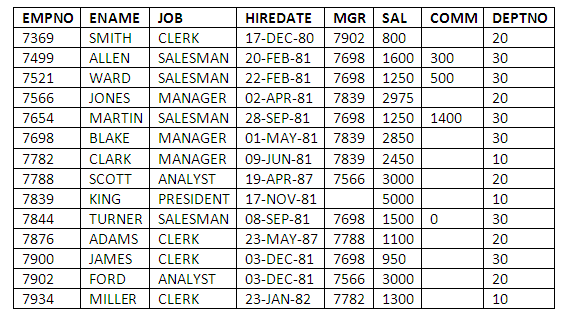
The EMP table stores records about company employees. This table defines and contains the values for the attributes EMPNO, ENAME, JOB, MGR, HIREDATE, SAL, COMM and DEPTNO.
EMPNO is a unique employee number; it is the primary key of the employee table.
ENAME stores the employee's name.
The JOB attribute stores the name of the job the employee does.
The MGR attribute contains the employee number of the employee who manages that employee. If the employee has no manager, then the MGR column for that employee is left set to null.
The HIREDATE column stores the date on which the employee joined the company.
The SAL column contains the details of employee salaries.
The COMM attribute stores values of commission paid to employees. Not all employees receive commission, in which case the COMM field is set to null.
The DEPTNO column stores the department number of the department in which each employee is based. This data item acts a foreign key, linking the employee details stored in the EMP table with the details of departments in which employees work, which are stored in the DEPT table.
The DEPT table stores records about the different departments that employees work in. This table defines and contains the values for the attributes as follows:
DEPTNO: The primary key containing the department numbers used to identify each department.
DNAME: The name of each department.
LOC: The location where each department is based.
The data in the EMP table contains the following 14 rows:
Figure 3.1
The DEPT table contains the following four rows:
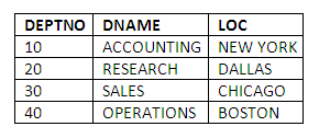
Figure 3.2
SQL queries can be written in upper or lower case, and on one or more lines. All queries in SQL begin with the word SELECT. The most basic form of the SELECT statement is as follows:
SELECT <select-list> FROM <table-list>
It is often useful to separate the different parts of a query onto different lines, so we might write this again as:
SELECT <select-list>
FROM <table-list>
Following the SELECT keyword is the list of table columns that the user wishes to view. This list is known as the select-list. As well as listing the table columns to be retrieved by the query, the select-list can also contain various SQL functions to process the data; for example, to carry out calculations on it. The select-list can also be used to specify headings to be displayed above the data values retrieved by the query. Multiple select-list items are separated from each other with commas. The select-list allows you to filter out the columns you don't want to see in the results.
The FROM keyword is, like the SELECT keyword, mandatory. It effectively terminates the select-list, and is followed by the list of tables to be used by the query to retrieve data. This list is known as the table-list. The fact that the tables need to be specified in the table-list means that, in order to retrieve data in SQL, you do need to know in which tables data items are stored. This may not seem surprising from the perspective of a programmer, or database developer, but what about an end-user? SQL has, in some circles, been put forward as a language that can be learned and used effectively by business users. We can see even at this early stage, however, that a knowledge of what data is stored where, at least at the logical level, is fundamental to the effective use of the language.
Exercise 1 - Fundamentals of SQL query statements
What keyword do all SQL query statements begin with?
What is the general form of simple SQL query statements?
Sample query 1 - the names of all employees
Suppose we wish to list the names of all employees. The SQL query would be:
SELECT ENAME
FROM EMP;
The single ENAME column we wish to see is the only entry in the select-list in this example. The employee names are stored in the EMP table, and so the EMP table must be put after the keyword FROM to identify from where the employee names are to be fetched.
Note that the SQL statement is terminated with a semi-colon (;). This is not strictly part of the SQL standard. However, in some SQL environments, it ensures that the system runs the query after it has been entered.
The result of this query when executed is as follows (note that your system might reflect this in a different way to what is shown here):
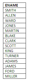
Figure 3.3
As you can see, the query returns a row for each record in the table, each row containing a single column presenting the name of the employee (i.e. the value of the DNAME attribute for each EMP record).
Sample query 2 - all data (rows and columns) from the DEPT table
There are two usual ways to list all data in a table. The simplest is to use a shorthand notation provided in SQL to list all the columns in any table. This is done simply by specifying an asterisk '*' for the select-list as follows:
SELECT *
FROM DEPT;
The asterisk is called a wild card, and causes all attributes of the specified table to be retrieved by the query.
Note that as it is the details of the DEPT table we wish to view, it is the DEPT table this time that appears in the table-list following the FROM keyword.
The use of * in this way is a very easy way to view the entire contents of any table. The alternative approach is simply to list all of the columns of the DEPT table in the select-list as follows:
SELECT DEPTNO, DENAME, LOC
FROM DEPT;
The result of executing either of these queries on our DEPT table at this time is the following:
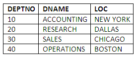
Figure 3.4
A potential problem of using the asterisk wild card, is that instead of explicitly listing all the attributes we want, the behaviour of the query will change if the table structure is altered — for example, if we add new attributes to the DEPT table, the SELECT * version of the query will then list the new attributes. This is a strong motivation for avoiding the use of the asterisk wild card in most situations.
Sample query 3 - the salary and commission of all employees
If we wish to see details of each employee’s salary and commission we would use the following query that specifies just those attributes we desire:
SELECT EMPNO, ENAME, SAL, COMM
FROM EMP;
In this example, we have included the EMPNO column, just in case we had any duplicate names among the employees.
The result of this query is:
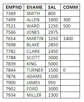
Figure 3.5
Sample query 4 - example calculation on a select-list
In the queries we have presented so far, the data we have requested has been one or more attributes present in each record. Following the principle of reducing data redundancy, many pieces of information that are useful, and that can be calculated from other stored data, are not stored explicitly in databases. SQL queries can perform a calculation 'on-the-fly' using data from table records to present this kind of information.
The salary and commission values of employees we shall assume to be monthly. Suppose we wish to display the total annual income (including commission) for each employee. This figure for each employee is not stored in the table, since it can be calculated from the monthly salary and commission values. The calculation is simply 12 times the sum of the monthly salary and commission.
A query that retrieves the number and name of each employee, and calculates their annual income, is as follows:
SELECT EMPNO, ENAME, 12 * (SAL + COMM)
FROM EMP;
The calculation here adds the monthly commission to the salary, and then multiplies the result by 12 to obtain the total annual income.
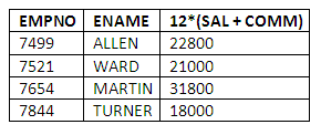
Figure 3.6
Notice that only records for which the commission value was not NULL have been included. This issue is discussion later in the chapter. When using some SQL implementation, such as MS Access, you may have to explicitly request records with NULL values to be excluded. So the above SQL query:
SELECT EMPNO, ENAME, 12 * (SAL + COMM)
FROM EMP;
may need to be written as:
SELECT EMPNO, ENAME, 12 * (SAL + COMM)
FROM EMP
WHERE COMM IS NOT NULL;
(See later to understand the WHERE part of this query)
Depending on which SQL system you run a query like this, the calculated column may or may not have a heading. The column heading may be the expression itself 12 * (SAL + COMM) or may be something indicating that an expression has been calculated: Expr1004 (these two examples are what happens in Oracle and MS Access respectively). Since such calculations usually mean something in particular (in this case, total annual income), it makes sense to name these calculated columns sensibly wherever possible.
Sometimes it is desirable to improve upon the default column headings for query results supplied by the system, to make the results of queries more intelligible. For example, the result of a query to calculate annual pay by summing the monthly salary and commission and multiplying by 12, would by default in some systems such as Oracle, have the expression of the calculation as the column heading. The result is more readable, however, if we supply a heading which clearly states what the compound value actually is, i.e. annual income. To do this, simply include the required header information, in double quotes, after the column specification in the select-list. For the annual pay example, this would be:
SELECT EMPNO, ENAME, 12*(SAL + COMM) "ANNUAL INCOME"
FROM EMP;
The result is more meaningful:
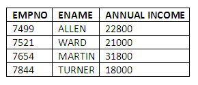
Figure 3.7
Once again, there are alternative ways to achieve the naming of columns in some systems including MS Access and MySQL, rather than using the double quotation marks around the column heading. The use of the keyword AS and square brackets may also be required.
So the SQL query:
SELECT EMPNO, ENAME, 12*(SAL + COMM) "ANNUAL INCOME"
FROM EMP;
may need to be written in as:
SELECT EMPNO, ENAME, 12*(SAL + COMM) AS ANNUAL INCOME
FROM EMP WHERE COMM IS NOT NULL;
(See next section to understand the WHERE part of this query)
Very often we wish to filter the records/rows retrieved by a query. That is, we may only wish to have a subset of the records of a table returned to us by a query.
The reason for this may be, for example, in order to restrict the employees shown in a query result just to those employees with a particular job, or with a particular salary range, etc. Filtering of records is achieved in SQL through the use of the WHERE clause. In effect, the WHERE clause implements the functionality of the RESTRICT operator from Relational Algebra, in that it takes a horizontal subset of the data over which the query is expressed.
The WHERE clause is not mandatory, but when it is used, it must appear following the table-list in an SQL statement. The clause consists of the keyword WHERE, followed by one or more restriction conditions, each of which are separated from one another using the keywords AND or OR.
The format of the basic SQL statement including a WHERE clause is therefore:
SELECT <select-list> FROM <table-list>
[WHERE <condition1> <, AND/OR CONDITION 2, .. CONDITION n>]
The number of conditions that can be included within a WHERE clause varies from DBMS to DBMS, though in most major commercial DBMS, such as Oracle, Sybase, Db2, etc, the limit is so high that it poses no practical restriction on query specifications. We can also use parentheses '(' and ')' to nest conditions or improve legibility.
WHERE example 1 - records with a value before some date
If we wish to retrieve all of those employees who were hired before, say, May 1981, we could issue the following query:
SELECT EMPNO, ENAME, HIREDATE
FROM EMP
WHERE HIREDATE < '01-MAY-1981';
The result of this query is:
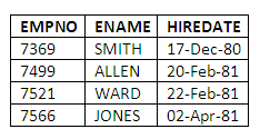
Figure 3.8
Note, incidentally, the standard form in which some systems such as Oracle handle dates: they are enclosed in single quotes, and appear as: DD-MMM-YYYY (two digits for day 'dd', three letters for month 'mmm' and four digits for year 'yyyy'). In some systems including MS Access, the date should be enclosed with two hash '#' characters, rather than single quotes - for example, #01-JAN-1990#. You should check with your system's documentation for the requirement as to how the dates should be formatted. Below are the two versions of the SQL statements, with different formats for dates:
For systems including Oracle:
SELECT EMPNO, ENAME, HIREDATE
FROM EMP
WHERE HIREDATE < '01-MAY-1981';
For systems including MS Access:
SELECT EMPNO, ENAME, HIREDATE
FROM EMP
WHERE HIREDATE < #01-MAY-1981#;
In our example above, we used the < (less than) arithmetic symbol to form the condition in the WHERE clause. In SQL, the following simple comparison operators are available:
= equals
!= is not equal to (allowed in some dialects)
< > is not equal to (ISO standard)
< = is less than or equal to
< is less than
> = is greater than or equal to
> is greater than
WHERE example 2 - two conditions that must both be true
The logical operator AND is used to specify that two conditions must both be true. When a WHERE clause has more than one condition, this is called a compound condition.
Suppose we wish to retrieve all salesmen who are paid more than 1500 a month. This can be achieved by ANDing the two conditions (is a salesman, and is paid more than 1500 a month) together in a WHERE clause as follows:
SELECT EMPNO, ENAME, JOB, SAL
FROM EMP
WHERE JOB = 'SALESMAN' AND SAL > 1500;
The result of this query is:
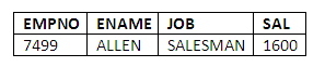
Figure 3.9
Only employees fulfilling both conditions will be returned by the query. Note the way in which the job is specified in the WHERE clause. This is an example of querying the value of a field of type character, or as it is called in Oracle, of type varchar2. When comparing attributes against fixed values of type character such as SALESMAN, the constant value being compared must be contained in single quotes, and must be expressed in the same case as it appears in the table. All of the data in the EMP and DEPT tables is in upper case, so when we are comparing character values, we must make sure they are in upper case for them to match the values in the EMP and DEPT tables. In other words, from a database point of view, the job values of SALESMAN and salesman are completely different, and if we express a data item in lower case when it is stored in upper case in the database, no match will be found.
In some systems, including MS Access, the text an attribute is to match should be enclosed with double quote characters, rather than single quotes. For example, "SALESMAN" rather than 'SALESMAN':
SELECT EMPNO, ENAME, JOB, SAL
FROM EMP
WHERE JOB = "SALESMAN" AND SAL > 1500;
WHERE example 3 - two conditions, one of which must be true
The logical operator OR is used to specify that at least one of two conditions must be true.
For example, if we wish to find employees who are based in either department 10 or department 20, we can do it by issuing two conditions in the WHERE clause as follows:
SELECT EMPNO, ENAME, DEPTNO
FROM EMP
WHERE DEPTNO = 10 OR DEPTNO = 20;
The result of this query is:
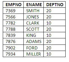
Figure 3.10
The keyword NOT can be used to negate a condition, i.e. only records that do not meet a condition are selected. An example might be to list all employees who are not salesmen:
SELECT EMPNO, ENAME, JOB, SAL
FROM EMP
WHERE NOT(JOB = 'SALESMAN');
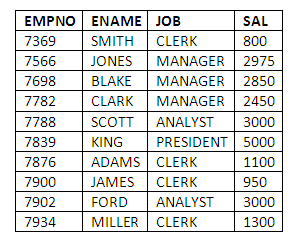
Figure 3.11
Another example might be to list all employees who do not earn more than 1500:
SELECT EMPNO, ENAME, JOB, SAL
FROM EMP
WHERE NOT(SAL > 1500 );
Figure 3.12
The operator != can be used to select where some value is NOT EQUAL TO some other value. So another way to write the query:
SELECT EMPNO, ENAME, JOB, SAL
FROM EMP
WHERE NOT(JOB = 'SALESMAN');
is as follows:
SELECT EMPNO, ENAME, JOB, SAL
FROM EMP
WHERE JOB != 'SALESMAN';
An alternative solution to the previous OR example is provided by a variation on the syntax of the WHERE clause, in which we can search for values contained in a specified list. This form of the WHERE clause is as follows:
WHERE ATTRIBUTE IN (<item1>, <item2>, ..., <itemN>)
Using this syntax, the previous query would be rewritten as follows:
SELECT EMPNO, ENAME, DEPTNO
FROM EMP
WHERE DEPTNO IN (10, 20);
The result of the query is just the same, but in many cases this form of the WHERE clause is both shorter and simpler to use.
The BETWEEN keyword can be used in a WHERE clause to test whether a value falls within a certain range. The general form of the WHERE clause using the BETWEEN keyword is:
WHERE <attribute> BETWEEN <value1> AND <value2>
The operands <value1> and <value2> can either be literals, like 1000, or expressions referring to attributes.
For example, if we wish to test for salaries falling in the range 1000 to 2000, then we can code as follows:
SELECT EMPNO, ENAME, SAL
FROM EMP
WHERE SAL BETWEEN 1000 AND 2000;
The result of this query is:
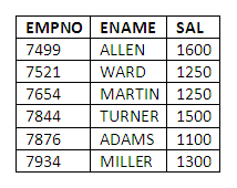
Figure 3.13
Note that the BETWEEN operator is inclusive, so a value of 1000 or 2000 would satisfy the condition and the record included in the query result.
An equally valid solution could have been produced by testing whether the salaries to be returned were >=1000 and <=2000, in which case, the WHERE clause would have been:
SELECT EMPNO, ENAME, SAL
FROM EMP
WHERE (SAL >=1000) AND (SAL <=2000);
However, this version of the query is longer and more complex, and includes the need to repeat the SAL attribute for comparison in the second condition of the WHERE clause.
In general, the solution using BETWEEN is preferable since it is more readable - it is clearer to a human reading the SQL query code what condition is being evaluated.
All of the queries we have seen so far have been to retrieve exact matches from the database. The LIKE keyword allows us to search for items for which we only know a part of the value. The LIKE keyword in SQL literally means 'is approximately equal to' or 'is a partial match with'. The keyword LIKE is used in conjunction with two special characters which can be used as wild card matches - in other words, LIKE expressions can be used to identify the fact that we do not know precisely what a part of the retrieved value is.
LIKE example - search for words beginning with a certain letter
As an example, we can search for all employees whose names begin with the letter S as follows:
SELECT EMPNO, ENAME
FROM EMP
WHERE ENAME LIKE 'S%'';
This query returns:
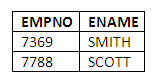
Figure 3.14
Here the percentage sign (%) is used as a wild card, to say that we do not know or do not wish to specify the rest of the value of the ENAME attribute; the only criteria we are specifying is that it begins with 'S', and it may be followed by no, one or more than one other character.
The percentage sign can be used at the beginning or end of a character string, and can be used as a wild card for any number of characters.
The other character that can be used as a wild card is the underline character (_). This character is used as a wild card for only one character per instance of the underline character. That is, if we code:
WHERE ENAME LIKE 'S__';
the query will return employees whose names start with S, and have precisely two further characters after the S. So employees called Sun or Sha would be returned, but employee names such as Smith or Salt would not be, as they do not contain exactly three characters.
Note that we can combine conditions using BETWEEN, or LIKE, with other conditions such as simple tests on salary, etc, by use of the keywords AND and OR, just as we can combine simple conditions. However, wild card characters cannot be used to specify members of a list with the IN keyword.
Data can very easily be sorted into different orders in SQL. We use the ORDER BY clause. This clause is optional, and when required appears as the last clause in a query. The ORDER BY keywords are followed by the attribute or attributes on which the data is to be sorted. If the sort is to be done on more than one attribute, the attributes are separated by commas.
The general form of an SQL query with the optional WHERE and ORDER BY clauses looks as follows:
SELECT <select-list> FROM <table-list>
[WHERE <condition1> <, AND/OR CONDITION 2, .. CONDITION n>] [ORDER BY <attribute-list>]
An example would be to sort the departments into department number order:
SELECT DEPTNO, DNAME
FROM DEPT
ORDER BY DEPTNO;
OR
SELECT DEPTNO, DNAME
FROM DEPT
ORDER BY DEPTNO ASC;
Note: SQL provides the keyword ASC to explicitly request ordering in ascending order.
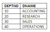
Figure 3.15
Or to sort into alphabetical order of the name of the department:
SELECT DEPTNO, DNAME
FROM DEPT
ORDER BY DNAME;
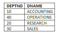
Figure 3.16
SQL provides the keyword DESC to request sorting in the reverse order. So to sort the departments into reverse alphabetical order, we can write the following:
SELECT DEPTNO, DNAME
FROM DEPT
ORDER BY DNAME DESC;
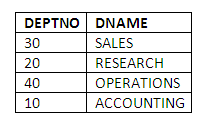
Figure 3.17
It is very easy to specify a sort within a sort, i.e. to first sort a set of records into one order, and then within each group to sort again by another attribute.
For example, the following query will sort employees into department number order, and within that, into employee name order.
SELECT EMPNO, ENAME, DEPTNO
FROM EMP
ORDER BY DEPTNO, ENAME;
The result of this query is:
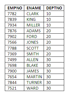
Figure 3.18
As can be seen, the records have been sorted into order of DEPTNO first, and then for each DEPTNO, the records have been sorted alphabetically by ENAME. This can be easily seen if you have a repeating DEPTNO - for example, if we had two employees, WARD and KUDO, belonging to DEPTNO 7521. Two DEPTNO 7521 will appear at the end of the table like above, but KUDO will be on top of WARD under the ENAME column.
When a query includes an ORDER BY clause, the data is sorted as follows:
Any null values appear first in the sort
Numbers are sorted into ascending numeric order
Character data is sorted into alphabetical order
Dates are sorted into chronological order
We can include an ORDER BY clause with a WHERE clause, as in the following example, which lists all salesman employees in ascending order of salary:
SELECT EMPNO,ENAME,JOB,SAL
FROM EMP
WHERE JOB = 'SALESMAN'
ORDER BY SAL;
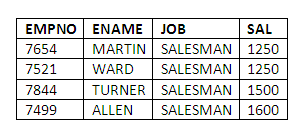
Figure 3.19
In the chapter introducing the Relational model, we discussed the fact that NULL values represent the absence of any actual value, and that it is correct to refer to an attribute being set to NULL, rather than being equal to NULL. The syntax of testing for NULL values in a WHERE clause reflects this. Rather than coding WHERE X = NULL, we write WHERE X IS NULL, or, WHERE X IS NOT NULL.
For example, to return all employees who do not receive a commission, the query would be:
SELECT EMPNO, ENAME, SAL
FROM EMP
WHERE COMM IS NULL;
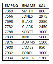
Figure 3.20
We can also select records that do not have NULL values:
SELECT EMPNO, ENAME, SAL, COMM
FROM EMP
WHERE COMM IS NOT NULL;
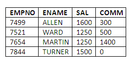
Figure 3.21
There is an extremely useful function available for the handling of NULLs in query results. (It is important to remember that NULL is not the same as, say, zero for a numeric attribute.) This is the NVL function, which can be used to substitute other values in place of NULLs in the results of queries. This may be required for a number of reasons:
By default, arithmetic and aggregate functions ignore NULL values in query results. Sometimes this is what is required, but at other times we might explicitly wish to consider a NULL in a numeric column as actually representing the value zero, for example.
We may wish to replace a NULL value, which will appear as a blank column in the displayed results of a query, with a more explicit indication that there was no value for that column instance.
The format of the NVL function is:
NVL(<column>, <value>)
<column> is the attribute in which NULLs are to be replaced, and <value> is the substitute value.
Examples of using the NVL function
An example of using NVL to treat all employees with NULL commissions as if they had zero commission:
SELECT EMPNO,NVL(COMM, 0)
FROM EMP;
To display the word 'unassigned' wherever a NULL value is retrieved from the JOB attribute:
SELECT EMPNO,NVL(job, 'unassigned')
FROM EMP;
Exercise
What would happen in the cases of employees who do not receive a commission, i.e. whose commission attribute is set to NULL?
Answer: The short, and somewhat surprising answer to this question, is that the records of employees receiving NULL commission will simply not be included in the result. The reason for this is that as we saw in the chapter on the Relational model, NULL simply indicates the absence of a real value, and so the result of adding a salary value to a NULL commission value is indeterminate. For this reason, SQL cannot return a value for the annual pay of employees where those employees receive no commission. There is a very useful solution to this problem, which will be dealt with later in this chapter, under the heading "Handling NULL values in query results”.
SQL functions help simplify different types of operations on the data. SQL supports four types of functions:
Arithmetic functions
Character functions
Date functions
Aggregate functions
The functions are used as part of a select-list of a query, or if they refer to a specific row, they may be used in a WHERE clause. They are used to modify the values or format of data being retrieved.
The most commonly used arithmetic functions are as follows:
greatest
greatest(object-list) - returns the greatest of a list of values
Example:
greatest(sal,comm) - returns whichever of the SAL or COMM attributes has the highest value
least
least(object-list) - returns the smallest of a list of values
Example:
least(sal,comm) - returns whichever of the SAL or COMM attributes has the lowest value
round
round(number[,d]) - rounds the number to d digits right of the decimal point (d can be negative)
Example:
round(sal,2) - rounds values of the SAL attribute to two decimal places
trunc
Trunc(number,d) – truncates number to d decimal places (d can be negative)
Example:
trunc(sal,2) - truncates values of the SAL attribute to two decimal places
Note: The difference between the round and truncate functions is that round will round up digits of five or higher, whilst trunc always rounds down.
abs
abs(number) - returns the absolute value of the number
Example:
abs(comm-sal) - returns the absolute value of COMM - SAL; that is, if the number returned would be negative, the minus sign is discarded
sign
sign(number) - returns 1 if number greater than zero, 0 if number = zero, -1 if number less than zero
Example:
sign(comm-sal) - returns 1 if COMM - SAL > 0, 0 if COMM - SAL = 0, and - 1 if COMM - SAL < 0
mod
mod(number1,number2) - returns the remainder when number1 is divided by number2
Example:
mod(sal,comm) - returns the remainder when SAL is divided by COMM
sqrt
sqrt(number) - returns the square root of the number. If the number is less than zero then sqrt returns null
Example:
sqrt(sal) - returns the square root of salaries
to_char
to_char(number[picture]) - converts a number to a character string in the format specified
Example:
to_char(sal,9999.99) - represents salary values with four digits before the decimal point, and two afterwards
decode
decode(column,starting-value,substituted-value..) - substitutes alternative values for a specified column
Example:
decode(comm,100,200,200,300,100) - returns values of commission increased by 100 for values of 100 and 200, and displays any other comm values as if they were 100
ceil
ceil(number) - rounds up a number to the nearest integer
Example:
ceil(sal) - rounds up salaries to the nearest integer
floor
floor(number) - truncates the number to the nearest integer
Example:
floor(sal) - rounds down salary values to the nearest integer
The most commonly used character string functions are as follows:
string1 || string2
string1 || string2 - concatenates (links) string1 with string2
Example:
deptno || empno - concatenates the employee number with the department number into one column in the query result
decode
decode(column,starting-value,substitute-value, ....) - translates column values to specified alternatives. The final parameter specifies the value to be substituted for any other values.
Example:
decode(job,'CLERK','ADMIN WORKER','MANAGER','BUDGET HOLDER',PRESIDENT','EXECUTIVE','NOBODY') This example translates values of the JOB column in the employee table to alternative values, and represents any other values with the string 'NOBODY'.
distinct
distinct <column> - lists the distinct values of the specific column
Example:
Distinct job - lists all the distinct values of job in the JOB attribute
length
length(string) - finds number of characters in the string
Example:
length(ename) - returns the number of characters in values of the ENAME attribute
substr
substr(column,start-position[,length]) - extracts a specified number of characters from a string
Example:
substr(ename,1,3) - extracts three characters from the ENAME column, starting from the first character
instr
instr(string1,string2[,start-position]) - finds the position of string2 in string1. The parentheses around the start-position attribute denote that it is optional
Example:
instr(ename,'S') - finds the position of the character 'S' in values of the ENAME attribute
upper
upper(string) - converts all characters in the string to upper case
Example:
upper(ename) - converts values of the ENAME attribute to upper case
lower
lower(string) - converts all characters in the string to lower case
Example:
lower(ename) - converts values of the ENAME attribute to lower case
to_number
to_number(string) - converts a character string to a number
Example:
to_number('11') + sal - adds the value 11 to employee salaries
to_date
to_date(str[,pict]) - converts a character string in a given format to a date
Example:
to_date('14/apr/99','dd/mon/yy') - converts the character string '14/apr/99' to the standard system representation for dates
soundex
soundex(string) - converts phonetically similar strings to the same value
Example:
soundex('smith') - converts all values that sound like the name Smith to the same value, enabling the retrieval of phonetically similar attribute values
vsize
vsize(string) - finds the number of characters required to store the character string
Example:
vsize(ename) - returns the number of bytes required to store values of the ENAME attribute
lpad
lpad(string,len[,char]) - left pads the string with filler characters
Example:
lpad(ename,10) - left pads values of the ENAME attribute with filler characters (spaces)
rpad
rpad(string,len[,char]) - right pads the string with filler characters
Example:
rpad(ename,10) - right pads values of the ENAME attribute with filler characters (spaces)
initcap
initcap(string) - capitalises the initial letter of every word in a string
Example:
initcap(job) - starts all values of the JOB attribute with a capital letter
translate
translate(string,from,to) - translates the occurrences of the 'from' string to the 'to' characters
Example:
translate(ename,'ABC','XYZ') - replaces all occurrences of the string 'ABC' in values of the ENAME attribute with the string 'XYZ'
ltrim
ltrim(string,set) - trims all characters in a set from the left of the string
Example:
ltrim(ename,' ') - removes all spaces from the start of values of the ENAME attribute
rtrim
rtrim(string,set) - trims all characters in the set from the right of the string
Example:
rtrim(job,'.') - removes any full-stop characters from the right-hand side of values of the JOB attribute
The date functions in most commercially available database systems are quite rich, reflecting the fact that many commercial applications are very date driven. The most commonly used date functions in SQL are as follows:
Sysdate Sysdate - returns the current date
add-months add-months(date, number) - adds a number of months from/to a date (number can be negative). For example: add-months(hiredate, 3). This adds three months to each value of the HIREDATE attribute
months-between months-between(date1, date2) - subtracts date2 from date1 to yield the difference in months. For example: months-between(sysdate, hiredate). This returns the number of months between the current date and the dates employees were hired
last-day last-day(date) - moves a date forward to last day in the month. For example: last-day(hiredate). This moves hiredate forward to the last day of the month in which they occurred
next-day next-day(date,day) - moves a date forward to the given day of week. For example: next-day(hiredate,'monday'). This returns all hiredates moved forward to the Monday following the occurrence of the hiredate
round round(date[,precision]) - rounds a date to a specified precision. For example: round(hiredate,'month'). This displays hiredates rounded to the nearest month
trunc trunc(date[,precision]) - truncates a date to a specified precision. For example: trunc(hiredate,'month'). This displays hiredates truncated to the nearest month
decode decode(column,starting-value,substituted-value) - substitutes alternative values for a specified column. For example: decode(hiredate,'25-dec-99','christmas day',hiredate). This displays any hiredates of the 25th of December, 1999, as Christmas Day, and any default values of hiredate as hiredate
to_char to_char(date,[picture]) - outputs the data in the specified character format. The format picture can be any combination of the formats shown below. The whole format picture must be enclosed in single quotes. Punctuation may be included in the picture where required. Any text should be enclosed in double quotes. The default date format is: 'dd-mon-yy'. Example: numeric format, description
cc, century, 20
y,yyy, year, 1,986
yyyy, year, 1986
yyy, last three digits of year, 986
yy, last two digits of year, 86
y, last digits of year, 6
q, quarter of year, 2
ww, week of year, 15
w, week of month, 2
mm, month, 04
ddd, day of year, 102
dd, day of month, 14
d, day of week, 7
hh or hh12, hour of day (01-12), 02
hh24, hour of day (01-24), 14
mi, minutes, 10
ss, seconds, 5
sssss, seconds past midnight, 50465
j, julian calendar day, 2446541
The following suffixes may be appended to any of the numeric formats (suffix, meaning, example):
th, st, nd, rd, after the number, 14th
sp, spells the number, fourteen
spth/st/nd/rd, spells the number, fourteenth
There is also a set of character format pictures (character format, meaning, example):
year, year, nineteen-eighty-six
month, name of month, april
mon, abbreviated month, apr
day, day of week, saturday
dy, abbreviated day, sat
am or pm, meridian indicator, pm
a.m. or p.m., meridian indicator, p.m.
bc or ad, year indicator, ad
b.c. or a.d., year indicator, a.d.
If you enter a date format in upper case, the actual value will be output in upper case. If the format is lower case, the value will be output in lower case. If the first character of the format is upper case and the rest lower case, the value will be output similarly.
For example:

to-char(hiredate,'dd/mon/yyyy')

to-char(hiredate,'day,"the"Ddspth"of"month')All aggregate functions with the exception of COUNT operate on numerical columns. All of the aggregate functions below operate on a number of rows:
avg
avg(column) - computes the average value and ignores null values
Example:
SELECT AVG(SAL) FROM EMP;
Gives the average salary in the employee table, which is 2073.21
Sum
Sum(column) - computes the total of all the values in the specified column and ignores null values
Example:
sum(comm) - calculates the total commission paid to all employees
min
min(column) - finds the minimum value in a column
Example:
min(sal) - returns the lowest salary
max
max(column) - finds the maximum value in a column
Example:
max(comm) - returns the highest commission
count
count(column) - counts the number of values and ignores nulls
Example:
count(empno) - counts the number of employees
variance
variance(column) - returns the variance of the group and ignores nulls
Example:
variance(sal) - returns the variance of all the salary values
Stddev
Stddev(column) - returns the standard deviation of a set of numbers (same as square root of variance)
Example:
stddev(comm) - returns the standard deviation of all commission values
Using the EMP and DEPT tables, create the following queries in SQL, and test them to ensure they are retrieving the correct data.
You may wish to review the attributes of the EMP and DEPT tables, which are shown along with the data near the start of the section called Introduction to the SQL language.
List all employees in the order they were hired to the company.
Calculate the sum of all the salaries of managers.
List the employee numbers, names and hiredates of all employees who were hired in 1982.
Count the number of different jobs in the EMP table without listing them.
Find the average commission, counting only those employees who receive a commission.
Find the average commission, counting employees who do not receive a commission as if they received a commission of 0.
Find in which city the Operations department is located.
What is the salary paid to the lowest-paid employee?
Find the total annual pay for Ward.
List all employees with no manager.
List all employees who are not managers.
How many characters are in the longest department name?
Distinguish between the select-list and the table-list in an SQL statement, explaining the use of each within an SQL statement.
What restrictions are there on the format and structure of the basic SQL queries as covered so far in this chapter? Describe the use of each of the major components of SQL query constructs that we have covered up to this point.
How are NULL values handled when data is sorted?
What facilities exist for formatting dates when output from an SQL statement?
What facilities are provided for analysing data in the same column across different rows in a table?
What is the role of the NVL function?
Is SQL for end-users?
As mentioned earlier in the chapter, a number of people in the database community believe that SQL is a viable language for end-users - that is, people whose jobs are not primarily involved with computing. From your introductory experience of the language so far, you should consider reasons for and against this view of the SQL language.
Can you think of any reasons why use of the wild card '*' as we have seen in a select-list may lead to problems?