Figure 5.1
Table of contents
At the end of this chapter you should be able to:
Create, alter and drop tables in SQL.
Insert, update and delete rows from SQL tables.
Create, alter and remove views based on SQL tables, and describe some of the strengths and limitations of views.
In parallel with this chapter, you should read Chapter 6 of Thomas Connolly and Carolyn Begg, "Database Systems A Practical Approach to Design, Implementation, and Management", (5th edn.).
This chapter introduces further features of the SQL language, and seeks to integrate the material of all three chapters which have provided coverage of SQL in this module. The chapter introduces the means by which tables are created, changed and removed in SQL. The statements for inserting, updating and deleting rows from tables are also covered. Views are an important feature in SQL for tailoring the presentation of data, and acting as a security mechanism. The statements for creating and using views will be described, along with some of the inherent limitations of the view mechanism.
This chapter is the final one specifically dedicated to the SQL language, and so it forms an important role in drawing together the information covered in all three of the SQL-related chapters of the module. SQL continues to be an important vehicle for explaining and illustrating concepts in many of the later chapters of the module, and provides a medium through which many relevant practical exercises can be performed.
Although this chapter is called Advanced SQL, the material covered is not in general more difficult than that of previous chapters. The previous two chapters on SQL have provided a fairly comprehensive coverage of the data manipulation (DML) part of the language, enabling the specification of a wide range of queries. This chapter introduces the mechanisms for creating, changing and removing tables, and for inserting, updating and removing rows from tables. The mechanisms for performing these actions in SQL are relatively straightforward, but are extremely powerful. Because SQL is a command-level language, these commands do not include the checks that we have grown to expect from a typical Graphical User Interface (GUI), and so they must be used with care.
Data definition language (DDL) statements are used for creating, modifying and removing data objects. They affect both physical and logical data structures. Their syntax is generally much more varied than the data manipulation language (DML) statements we have covered in the previous two chapters.
The CREATE statement in SQL can be used to bring into being a range of different data objects, including the following:
Data tables
Views on existing tables
Indexes (data structures which speed up access to data)
Database user accounts
In this section we shall concentrate on the use of the CREATE statement for establishing new tables. The CREATE TABLE statement has a range of different options, and so we shall start by showing a simplified version of the syntax as follows:
CREATE TABLE "TABLE NAME" (COLUMN SPECIFICATION 1, ...... COLUMN SPECIFICATION n);
Where column specification includes:
A column name
The data type of the column
Where appropriate, a specification of the length of the column
An optional indicator of whether or not the column is to contain null values
Data objects are subject to a number of restrictions, and these will vary between different database systems. We shall describe the restrictions on naming tables and columns in Oracle, as they are fairly typical limitations encountered in databases generally, the main exceptions being older PC-based database environments.
Table names must start with an alphabetic character, and can contain up to 30 characters.
Table names can contain the letters A-Z, the numbers 0-9, and the characters – and _.
Table names must be unique within any specific user account.
Column names must start with a character, and may comprise up to 30 characters.
They can contain the same characters as table names.
Column names must be unique within a table, but you can specify the same column names in different tables.
In Oracle there can be up to 254 columns in a table.
Referring to the simplified version of the CREATE TABLE statement above, the column specifications are contained in parentheses.
We shall focus on three specific data types for use in our practical work, as their equivalents (though they may be differently named) can be found in almost any database environment. These data types appear in Oracle as the following:
VARCHAR2 (length)
where length is the maximum length of the character string to be stored.
Note: Some DBMSs, including MySQL, uses VARCHAR instead.
NUMBER (precision, scale)
where precision is the maximum number of digits to be stored and scale indicates number of digits to the right of the decimal point. If scale is omitted, then integer (whole) numbers are stored.
Note: Some DBMSs, including MySQL, expect you to use exact data types for numeric data. For example, if you want to hold integers, then you must use the INT datatype. If you wish to hold decimal numbers, then you must use the DOUBLE datatype.
Like many other systems, Oracle contains a number of other data types in addition to the most commonly found ones just described. As an example of other data types that may be provided, here are a few of the rather more Oracle-specific data types available:
Decimal: is used to store fixed-point numbers, and provides compatibility with IBM’s DB2 and SQL/DS systems.
Float: is used to store floating-point numbers, and provides compatibility with the ANSI float datatype.
Char: is used to store fixed-length character strings. It is most commonly used for representing attributes of one character in length.
Long: is used to store a little over two gigabytes of data. However, none of Oracle’s built-in functions and operators can be used to search an attribute of type 'long'.
The final part of a column specification allows us to specify whether or not the column is to contain null values, i.e. whether or not it is a mandatory column. The syntax is simply to specify either "Not null" or Null after the data type (and possible length) specification.
Example CREATE TABLE statement
Suppose we wished to create a table called MUSIC_COLLECTION, which we would use to store the details of CDs, cassettes, minidiscs, etc. This could be done with the following statement:
CREATE TABLE MUSIC_COLLECTION (ITEM_ID NUMBER(4),
TITLE VARCHAR2(40),
ARTIST VARCHAR2(30),
ITEM_TYPE VARCHAR2(1),
DATE_PURCHASED DATE);
We use a unique numeric identifier called ITEM_ID to identify each of the items in the collection, as we cannot rely on either the TITLE or ARTIST attributes to identify items uniquely. The ITEM_TYPE attribute is used to identify which format the item is in, i.e. cassette, CD, etc.
Remember that a primary key is used to identify uniquely each instance of an entity. For the MUSIC_COLLECTION table, the primary key of ITEM_ID will identify uniquely each of the items in the music collection. The CREATE TABLE statement provides the syntax to define primary keys as follows:
CREATE TABLE "TABLE NAME"
(COLUMN SPECIFICATION 1,
COLUMN SPECIFICATION n,
PRIMARY KEY (columnA, ...., columnX));
where columns columnA,....,columnX are the columns to be included in the primary key, separated from each other by commas, and all of the columns included in the primary key being enclosed in parentheses. In SQL the definition of a primary key on a CREATE TABLE statement is optional, but in practice this is virtually always worth doing. It will help maintain the integrity of the database. Oracle will ensure all the values of a primary key are different, and will not allow a null value to be entered for a primary key. In Oracle there is an upper limit of 16 columns that can be included within a primary key.
Example of creating table with a primary key
If we wanted to specify that ITEM_ID is to be used as the primary key in the MUSIC-COLLECTION table, we could code the following version of our CREATE TABLE statement:
CREATE TABLE MUSIC_COLLECTION (ITEM_ID NUMBER(4),
TITLE VARCHAR2(40),
ARTIST VARCHAR2(30), ITEM_TYPE VARCHAR2(1),
DATE_PURCHASED DATE, PRIMARY KEY (ITEM_ID));
A foreign key is used to form the link between rows stored in one table and corresponding rows in another table. For example, in the sample data set we have used in the previous two chapters on SQL, the foreign key EMP.DEPTNO in the employee table was used to link employees to their corresponding departments in the DEPT table. The CREATE TABLE statement allows us to specify one or more foreign keys in a table as follows:
CREATE TABLE "TABLE NAME"
(COLUMN SPECIFICATION 1,
COLUMN SPECIFICATION n,
PRIMARY KEY (columnA, ...., columnX), CONSTRAINT "constraint name"
FOREIGN KEY (columnAA, ...., columnXX) REFERENCES "primary key specification")
...............);
As for primary keys, foreign key specifications are not mandatory in a CREATE TABLE statement. But again, specifying foreign keys is desirable in maintaining the integrity of the database. Oracle will ensure that a value entered for a foreign key must either equal a value of the corresponding primary key, or be null. CREATE TABLE statements can contain both a primary key specification, and a number of foreign key specifications.
An explanation of the foreign key specification is as follows:
The first item is the keyword "CONSTRAINT", followed by an optional constraint name. Although specifying a constraint name is optional, it is recommended that you always include it. The reason for this is that if no constraint name is specified, most systems, including Oracle, will allocate one, and this will not be in any way easy to remember. If you later wish to refer to the foreign key constraint - for instance, because you wish to remove it - then providing your own name at the point you enter the CREATE TABLE statement will make this much easier.
The words FOREIGN KEY are followed by a list of the columns to be included in the foreign key, contained in parentheses and separated by commas (this list of column names is in general different from the list of column names in the "Primary key" clause).
REFERENCES is the mandatory keyword, indicating that the foreign key will refer to a primary key.
The primary key specification starts with the name of the table containing the referenced primary key, and then lists the columns comprising the primary key, contained in parentheses and separated by commas as usual.
The full stops (...............) shown in the version of the syntax above indicate that there may be more than one foreign key specification.
Example of defining a foreign key in SQL
Supposing we have a second table, which we use to keep track of recording artists whose recordings we buy. The ARTIST table could be created with the following statement:
CREATE TABLE ARTIST (
ARTIST_ID NUMBER(2),
ARTIST_NAME VARCHAR2(30),
COUNTRY_OF_ORIGIN VARCHAR2(25),
DATE_OF_BIRTH DATE, PRIMARY KEY (ARTIST_ID));
To relate the MUSIC_COLLECTION table to the ARTIST table, we could make the following modifications to the CREATE TABLE statement for the MUSIC_COLLECTION TABLE, which replaces the ARTIST_NAME with a foreign key reference to the ARTIST-ID:
CREATE TABLE MUSIC_COLLECTION (ITEM_ID NUMBER(4),
TITLE VARCHAR(40),
ARTIST_ID NUMBER(2),
ITEM_TYPE VARCHAR2(1),
DATE_PURCHASED DATE, PRIMARY KEY (ITEM_ID),
CONSTRAINT FK_ARTIST
FOREIGN KEY (ARTIST_ID) REFERENCES ARTIST (ARTIST_ID));
The following points should be noted:
We have modified the attribute specified on line four, from containing the Artist name, and being of type Varchar2 and length 30, to be the ARTIST_ID, of type number and length2.
We have then used the ARTIST_ID as the foreign key, which references the primary key of the table ARTIST.
Note that in general, it would not be possible to make changes such as these to existing tables. It would require some existing tables and data to be deleted. Therefore it is good practice to consider very carefully the design of tables and specification of the primary and foreign keys that are going to be required, and to specify this correctly the first time in CREATE TABLE statements. It is however possible to add and remove both primary key and foreign key constraints, and this will be covered, along with the details of a range of other constraints mechanisms, in the chapter Declarative Constraints and Database Triggers.
An extremely useful variant of the CREATE TABLE statement exists for copying data. Essentially, this consists of using a SELECT statement to provide the column specifications for the table to be created and, in addition, the data that is retrieved by the SELECT statement is copied into the new table structure. The syntax for this form of the statement is as follows:
CREATE TABLE "TABLE NAME"
AS "select statement";
where "select statement" can be any valid SQL query.
This form of the CREATE TABLE statement can be used to, for example:
Copy entire tables.
Copy subsets of tables using the select-list and WHERE clause to filter rows.
Create tables which combine data from more than one table (using JOINs).
Create tables containing aggregated data (using GROUP BY).
Examples of copying data using CREATE TABLE.....SELECT
Example 1:
To create a copy of the EMP table we have used in previous exercises:
CREATE TABLE EMPCOPY
AS SELECT * FROM EMP;
Example 2:
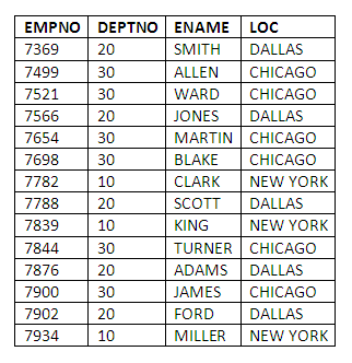
To create a table containing a list of employees and their locations we can code:
CREATE TABLE EMPLOC
AS SELECT EMPNO, EMP.DEPTNO, ENAME, LOC
FROM EMP, DEPT
WHERE EMP.DEPTNO = DEPT.DEPTNO;
To examine the contents of the new table:
SELECT *
FROM EMPLOC;
Figure 5.1
Sometimes you may wish to copy the structure of a table without moving any of the data from the old table into the new one. For example, to take a copy of the structure of the EMP table, but without copying any employee records into the new table, we could use:
CREATE TABLE EMPSTRUCT
AS SELECT *
FROM EMP
WHERE 1 = 2;
To verify we have copied the structure:
DESCRIBE EMPSTRUCT
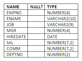
Figure 5.2
To verify the new structure contains no data:
SELECT *
FROM EMPSTRUCT;
no rows selected
This is an example of the way the SQL language can be made to fit a particular purpose. We wish in this example to copy the structure of a table, but ensure no rows are selected from it. By supplying a WHERE clause which contains a condition, namely WHERE 1 = 2, that can never be satisfied, we ensure that no rows are copied along with the structure.
The ALTER statement in SQL, like the CREATE statement, can be used to change a number of different types of data objects, including tables, access privileges and constraints. Here we shall concentrate on its use to change the structure of tables.
You can use the ALTER TABLE statement to modify a table's definition. This statement changes the structure of a table, not its contents. You can use the ALTER TABLE statement to:
Add a new column to an existing table.
Increase or decrease the width of an existing column.
Change an existing column from mandatory to optional (i.e. specify that it may contain nulls).
Columns can be added to existing tables with this form of the ALTER TABLE statement. The syntax is:
ALTER TABLE "TABLE NAME"
ADD "COLUMN SPECIFICATION 1",
............,
"COLUMN SPECIFICATION n";
For example, to add a department-head attribute to the DEPT table, we could specify:
ALTER TABLE DEPT
ADD DEPT_HEAD NUMBER(4);
We could imagine that the new DEPT_HEAD column would contain EMPNO values, corresponding to the employees who were the department heads of particular departments. Incidentally, if we had wished to make the DEPT_HEAD field mandatory, we could not have done so, as the ALTER TABLE statement does not enable the addition of mandatory fields to tables that already contain data.
We can add a number of columns with one ALTER TABLE statement.
This form of the ALTER TABLE statement permits changes to be made to existing column definitions. The format is:
ALTER TABLE "TABLE NAME"
MODIFY "COLUMN SPECIFICATION 1",
.............,
COLUMN SPECIFICATION n";
For example, to change our copy of the EMP table, called EMPCOPY, so that the DEPTNO attribute can contain three digit values:
ALTER TABLE EMPCOPY
MODIFY DEPTNO NUMBER(3);
This form of the ALTER TABLE statement can be used to:
Increase the length of an existing column.
Transform a column from mandatory to optional (i.e. specify it can contain nulls).
There are a number of restrictions in the use of the ALTER TABLE statement for modifying columns, most of which might be guessed through a careful consideration of what is being required of the system. For example, you cannot:
Reduce the size of an existing column (even if it has no data in it).
Change a column from being optional to mandatory.
To remove a table, the DDL statement is:
DROP TABLE "TABLE NAME";
It is deceptively easy to issue this command, and unlike most systems one encounters today, there is no prompt at all about whether you wish to proceed with the process. Dropping a table involves the removal of all the data and constraints on the table and, finally, removal of the table structure itself.
Example to remove our copy of the EMP table, called EMPCOPY:
DROP TABLE EMPCOPY;
Table dropped.
Sometimes we wish to recreate an existing table, perhaps because we wish to add new constraints to it, or to carry out changes that are not easy to perform using the ALTER TABLE or other DDL statements. If this is the case, it will be necessary to drop the table before issuing the new CREATE TABLE statement. Clearly this should only be done if the data in the table can be lost, or can be safely copied elsewhere, perhaps through the use of a CREATE TABLE with a SELECT clause.
For a little further information about the use of the DROP TABLE statement when creating tables, see the section on using SQL scripts later in this chapter.
The INSERT statement is used to add rows to an existing table. The statement has two basic forms:
INSERT INTO "TABLE NAME" (COLUMN-LIST) VALUES
(LIST OF VALUES TO BE INSERTED);
The COLUMN-LIST describes all of the columns into which data is to be inserted. If values are to be inserted for every column, i.e. an entire row is to be added, then the COLUMN-LIST can be omitted.
The LIST OF VALUES TO BE INSERTED comprises the separate values of the new data items, separated by commas.
Example 1:
To insert a new row into the table DEPTCOPY (this is a copy of the DEPT table):
INSERT INTO DEPTCOPY VALUES (50,'PURCHASING','SAN FRANCISCO');
1 row created.
Example 2:
To insert a new department for which we do not yet know the location:
INSERT INTO DEPTCOPY (DEPTNO,DNAME)
VALUES (60,'PRODUCTION');
1 row created.
The syntax for this form of the INSERT statement is as follows:
INSERT INTO "TABLE NAME" (COLUMN-LIST)
"SELECT STATEMENT";
The COLUMN-LIST is optional, and is used to specify which columns are to be filled when not all the columns in the rows of the target table are to be filled.
The "SELECT STATEMENT" is any valid select statement.
This is, rather like the case of using SELECT with the CREATE TABLE statement, a very powerful way of moving existing data (possibly from separate tables) into a new table.
Example:
Supposing we have created a table called MANAGER, which is currently empty. To insert the numbers, names and salaries of all the employees who are managers into the table we would code:
INSERT INTO MANAGER
SELECT EMPNO, ENAME, SAL
FROM EMP
WHERE JOB = 'MANAGER';
3 rows created.
To verify the employees in the table are managers, we can select the data and compare the jobs of those employees in the original EMP table:
SELECT *
FROM MANAGER;
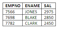
Figure 5.3
The UPDATE statement is used to change the values of columns in SQL tables. It is extremely powerful, but like the DROP statement we encountered earlier, it does not prompt you about whether you really wish to make the changes you have specified, and so it must be used with care.
The syntax of the UPDATE statement is as follows:
UPDATE "TABLE NAME" SET "column-list" = expression | sub-query WHERE "CONDITION";
The SET keyword immediately precedes the column or columns to be updated, which are specified in the column list. If there is more than one column in the list, they are separated by commas.
Following the equals sign "=" there are two possibilities for the format of the value to be assigned. An expression can be used, which may include mathematical operations on table columns as well as constant values. If an expression is supplying the update value, then only one column can be updated.
Alternatively, a sub-query or SELECT statement can be used to return the value or values to which the updated columns will be set. If a sub-query is used to return the updated values, then the number of columns to be updated must be the same as the number of columns in the select-list of the sub-query.
Finally, the syntax includes a WHERE clause, which is used to specify which rows in the target table will be updated. If this WHERE clause is omitted, all rows in the table will be updated.
Example 1:
To give all the analysts in the copy of the EMP table (called EMPCOPY) a raise of 10%:
UPDATE EMPCOPY
SET SAL = SAL * 1.1
WHERE JOB = 'ANALYST';
2 rows updated.
Example 2:
Suppose we wish to flatten the management structure for the employees stored in the EMPCOPY table. Recall that the MGR of each employee contains the employee number of their manager. We might implement this flattening exercise, at least as far as the database systems are concerned, by setting all employees' MGR fields to that of KING, who is the president of the company. The update statement to do this would be as follows:
UPDATE EMPCOPY
SET MGR =
(SELECT EMPNO
FROM EMP
WHERE ENAME = 'KING') WHERE ENAME != 'KING';
13 rows updated.
Note that we have been careful to include the final WHERE clause, in this case to avoid updating KING’s MGR field.
To verify that the updates have taken place correctly:
SELECT EMPNO,ENAME,MGR
FROM EMPCOPY;
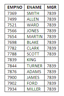
Figure 5.4
Note that all MGR fields, except that of KING, have been set to 7839, which is of course KING’s EMPNO. It is a nice feature of the SQL language that we were able to code this query without knowing KING’s EMPNO value, though we did have to know something unique about KING in order to retrieve the EMPNO value from the table. In this case, we used the value of ENAME, but this is in general unsafe - it would have been better to use KING’s EMPNO value. Why? We could equally have used the value of JOB, providing we could rely on there being only one President in the table.
The DELETE statement is the last of the DDL statements we shall look at in detail. It is used to remove single rows or groups of rows from a table. Its format is as follows:
DELETE FROM "TABLE NAME"
WHERE "COLUMN-LIST" = | IN
CONSTANT | EXPRESSION | SUB-QUERY;
As for the UPDATE statement, if the WHERE clause is omitted, all of the rows will be removed from the table. However, unlike the DROP TABLE statement, a DELETE statement leaves the table structure in place.
Example 1: To remove an individual employee from the EMPCOPY table:
DELETE FROM EMPCOPY
WHERE ENAME = 'FORD';
1 row deleted.
Note that, had there been more than one employee called FORD, all would have been deleted.
Example 2: To delete a number of rows based on an expression: To remove all employees paid more than 2800:
DELETE FROM EMPCOPY
WHERE SAL > 2800;
5 rows deleted.
Example 3: Deleting using a sub-query: To remove any employees based in the SALES department:
DELETE FROM EMPCOPY
WHERE DEPTNO IN
(SELECT DEPTNO FROM DEPT WHERE DNAME = 'SALES');
5 rows deleted
Views are an extremely useful mechanism for providing users with a subset of the underlying data tables. As such, they can provide a security mechanism, or simply be used to make the user’s job easier by reducing the rows and columns of irrelevant data to which users are exposed.
Views are the means by which, in SQL databases, individual users are provided with a logical, tailored schema of the underlying database. Views are in effect virtual tables, but appear to users in most respects the same as normal base tables. The difference is that when a view is created, it is not stored like a base table; its definition is simply used to recreate it for use each time it is required. In this sense, views are equivalent to stored queries.
Views are created using the CREATE VIEW statement. The syntax of this statement is very similar to that for creating tables using a SELECT.
Example: To create a view showing the names and hiredates of employees, based on the EMP table:
CREATE VIEW EMPHIRE
AS SELECT ENAME,HIREDATE
FROM EMP;
View created.
To examine the structure of the view EMPHIRE, we can use the DESCRIBE command, just as for table objects:
DESCRIBE EMPHIRE
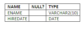
Figure 5.5
To see the data in the view, we can issue a SELECT statement just as if the view EMPHIRE is a table:
SELECT *
FROM EMPHIRE;
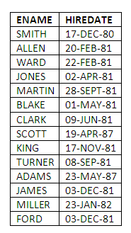
Figure 5.6
When specifying the rows and columns to be included in a view definition, we can use all of the facilities of a SELECT statement. However, there are a number of situations in which the data in base tables cannot be updated via a view. These are as follows:
When the view is based on one table, but does not contain the primary key of the table.
When the view is based on a JOIN.
When a view is based on a GROUP BY clause or aggregate function, because there is no underlying row in which to place the update.
Where rows might migrate in or out of a view as a result of the update being made.
The syntax of this extremely useful command is as follows:
RENAME "old table name" TO "new table name";
Example: to rename the EMP table to NEWEMP:
RENAME EMP TO NEWEMP;
Table renamed.
The RENAME command is an extremely useful one when carrying out DDL operations. This is in part because of the shortcomings of the ALTER TABLE statement, which makes it necessary sometimes to copy a sub- or super-set of the table, drop the former version of the table, and rename the new version to the old.
For example, if we wish to remove a column from a table, it is necessary to do the following:
Use the CREATE TABLE statement to make a copy of the old table, excluding the column which is no longer required.
Drop the old copy of the table.
Rename the new copy of the table to the old.
SQL allows us to create and drop a database in an easy way.
Creating a database uses the following syntax:
CREATE SCHEMA database-name;
For example, to create a database called STUDENTS that holds student information, we write the create command as follows:
CREATE SCHEMA students;
Deleting the database is also fairly easy:
DROP SCHEMA database-name;
For example, to delete the student database, we write the delete command as follows:
DROP SCHEMA students;
Warning: Be careful when using the DROP SCHEMA command. It deletes all the tables created under that database, including the data.
SQL statements can be combined into a file and executed as a group. This is particularly useful when it is required to create a set of tables together, or use a large number of INSERT statements to enter rows into tables. Files containing SQL statements in this way are called SQL script files. Each separate SQL statement in the file must be terminated with a semi-colon to make it run. Comments can be included in the file with the use of the REM statement, e.g.
REM insert your comment here
The word REM appears at the start of a new line in the script file. REM statements do not require a semi-colon (;) terminator.
Having created one or more tables, if you then decide you wish to make changes to them, some of which may be difficult or impossible using the ALTER TABLE statement, the simplest approach is to drop the tables and issue a new CREATE TABLE statement which implements the required changes. If the tables whose structures you wish to change contain any data you wish to retain, you should first use CREATE TABLE with a sub-query to copy the data to another table, from which it can be copied back when you have carried out the required table restructuring.
The restructuring of a number of tables is best implemented by including the required CREATE TABLE statements in a script file. To avoid errors when this file is re-run, it is customary to place a series of DROP TABLE statements at the beginning of the file, one for each table that is to be created. In this way you can re-run the script file with no problems. The first time it runs, assuming the tables have not already been created outside the script, the DROP TABLE statements will raise error messages, but these can be ignored. It is of course essential, if the tables contain data, to ensure this has been copied to other tables before such a restructuring exercise is undertaken.
Tables:
TUTOR (TUTOR_ID, TUTOR_NAME, DEPARTMENT, SALARY, ADVICE_TIME)
STUDENT(STUDENT_NO, STUDENT_NAME, DATE_JOINED, COURSE, TUTOR_ID)
Important note: Because of the foreign key constraint, you should create the TUTOR table first, so that it will be available to be referenced by the foreign key from the STUDENT table when it is created.
Use DESCRIBE to check the table structure.
Add an ANNUAL_FEE column to the STUDENT table.
Ensure that the STUDENT_NO field is sufficiently large to accommodate over 10,000 students. If it is not, change it so that it can deal with this situation.
Add an ANNUAL_LEAVE attribute to the tutor table.
Ensure that the tutor’s salary attribute can handle salaries to a precision of two decimal places. Remove the ADVICE_TIME attribute from the tutor table.
INSERT INTO STUDENT VALUES (1505,'KHAN','04-OCT-1999','COMPUTING',NULL,5000);
1 row created.
Note that because inserting data a row at a time with the INSERT statement is rather slow, it is only necessary to put small samples of tutors and students into the tables; for example, about four tutor records and eight student records should be sufficient.
Use CREATE TABLE with a sub-query to make copies of your TUTOR and STUDENT tables before you proceed to the following steps of the activity, which involve updating and removing data. Having done this, if you accidentally remove more data than you intended, you can copy it back from your backup tables by dropping the table, and then using the CREATE TABLE statement with a sub-query.
Update a specific student record in order to change the course he or she is attending.
Update the TUTOR_ID of a specific student in order to change the tutor for that student. Write the update statement by using the tutor’s name, in order to retrieve the TUTOR_ID supplying the update value.
Remove all students who do not have a tutor.
View1 should contain details of all students taking Computing.
View2 should include the names of tutors and the names of their tutees.
Describe the ways in which tables can be created in SQL.
What details need to be included on a CREATE TABLE statement to establish a foreign key?
Briefly describe the functionality of the ALTER TABLE statement, and describe some of the limitations in its use.
What happens to the data in a table when that table is dropped?
Describe the forms that the INSERT statement can take.
What options are there for supplying values to update columns in an UPDATE statement?
What happens to a table structure when rows are deleted from the table?
The command-oriented nature of the SQL language means that it does not contain the usual confirmation messages if requests are made to remove data or storage structures such as tables. Identify the SQL statements where it is necessary to pay particular attention to the statement specification, in order to avoid unwanted changes to data or data structures. Identify which parts of the statements require specific attention in this way.
Describe two uses of views in database systems, and identify any limitations in their use.
The strengths and weaknesses of SQL
The three chapters covering SQL have introduced a wide range of mechanisms for querying and manipulating data in relational tables. This is not the complete story as far as SQL is concerned, but you have now encountered a major part of the facilities available within standard implementations of the language. You are encouraged to discuss with your colleagues your views on the SQL language that you have been learning. Particular aspects of interest for discussion include:
What do you feel are the strengths of the language, in terms of learnability, usability and flexibility?
On the other hand, which aspects of the language have you found difficult or awkward either to learn or to use?
Are there ways in which you feel the language could be improved?
How does use of the SQL language compare with other database systems or programming languages you have encountered?
How feasible is it to use natural language (e.g. English) statements instead of SQL, to retrieve data in an Oracle database? What are the potential problems and how might they be overcome?
The SQL language, as we have seen, provides a standardised, command-based approach to the querying and manipulation of data. Most database systems also include Graphical User Interfaces for carrying out many of the operations that can be performed in SQL. You are encouraged to explore these interfaces, either for the Microsoft Access database system, and/or for the Personal Oracle system you have installed to carry out the practical work so far.
The Microsoft Access system does not provide the DDL part of SQL, relying on its graphical front-end for the creation and alteration of tables. Examine the ways in which new tables are established or changed within the Microsoft Access environment, comparing it with the approach in SQL.
The Personal Oracle system includes a graphical tool called the Navigator, which provides a graphical means of carrying out a large number of database administration tasks.
Examine the facilities in the Navigator for creating tables and other data objects, again comparing it with the equivalent mechanisms in SQL.