Figure 4.1
Table of contents
At the end of this chapter you should be able to:
Group and summarise data together.
Combine the grouping mechanisms with the aggregation functions covered in the previous chapter to provide useful summarised reports of data.
Write queries that retrieve results by combining information from a number of tables.
Combine the results of multiple queries in various ways.
In parallel with this chapter, you should read Chapter 5 of Thomas Connolly and Carolyn Begg, "Database Systems A Practical Approach to Design, Implementation, and Management", (5th edn.).
This chapter builds on the foundations laid in the previous chapter, which introduced the SQL language. We examine a range of facilities for writing more advanced queries of SQL databases, including queries on more than one table, summarising data, and combining the results of multiple queries in various ways.
This chapter forms the bridge between the chapter in which the SQL language was introduced, and the coverage of the data definition language (DDL) and data control language (DCL) provided in the next chapter called Advanced SQL.
It is possible to express a range of complex queries using the data manipulation language (DML) previously introduced. The earlier chapter showed how fairly simple queries can be constructed using the select-list, the WHERE clause to filter rows out of a query result, and the ORDER BY clause to sort information. This chapter completes the coverage of the DML facilities of SQL, and will considerably increase the range of queries you are able to write. The final SQL chapter will then address aspects of SQL relating to the updating of data and the manipulation of the logical structures, i.e. tables that contain data.
Information retrieved from an SQL query can very easily be placed into separate groups or categories by use of the GROUP BY clause. The clause is similar in format to ORDER BY, in that the specification of the words GROUP BY is followed by the data item or items to be used for forming the groups. The GROUP BY is optional. If it appears in the query, it must appear before the ORDER BY if the ORDER BY is present.
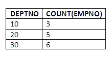
Example: count the number of employees in each department
To answer this question, it is necessary to place the employees in the EMP table into separate categories, one for each department. This can be done easily enough through the use of the DEPTNO column in the EMP table as follows (with the select-list temporarily omitted):
SELECT ….
FROM EMP
GROUP BY DEPTNO
As far as counting the employees is concerned, this is an example of something that is seen very commonly with the GROUP BY clause; that is, the use of an aggregation function, in this case the COUNT function, in conjunction with GROUP BY. To complete the query, we simply need to include on the select-list the DEPTNO column, so that we can see what we are grouping by, and the COUNT function. The query then becomes:
SELECT DEPTNO,COUNT(EMPNO)
FROM EMP
GROUP BY DEPTNO;
Figure 4.1
Comments: The query works in two steps. The first step is to group all employees by DEPTNO. The second step is to count the number of employees in each group. Of course, headings could be used to improve the clarity of the results; for example, specifying that the second column is “no. of employees”.
COUNT(EMPNO) AS no. of employeesWe have specified between the parentheses of the COUNT function that we are counting EMPNOs, because we are indeed counting employees. We could in fact have merely specified an asterisk, “*” in the parentheses of the COUNT function, and the system would have worked out that we were counting instances of records in the EMP table, which equates to counting employees. However, it is more efficient to specify to the system what is being counted.
GROUP BY, like ORDER BY, can include more than one data item, so for example if we specify:
GROUP BY DEPTNO, JOB
the results will be returned initially categorised within departments, and then within that, categorised into employees who do the same job.
GROUP BY example
Find the average salary for each JOB in the company:
SELECT JOB, AVG(round(SAL,2))
FROM EMP
GROUP BY JOB;
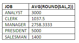
Figure 4.2
Comments: This is a fairly straightforward use of the GROUP BY clause, once again in conjunction with an aggregate function, AVG.
All column names in the select-list must appear in the GROUP BY clause, unless the name is used only in an aggregate function. Many people when first starting to use the GROUP BY clause, fall into the trap of asking the system to retrieve and display information at two different levels. This arises if, for example, you GROUP BY a data item such as JOB, but then on the select-list, include a data item at the individual employee level, such as HIREDATE, SAL, ETC. You might think that we displayed salaries in the previous example, where we listed the average salaries earned by employees doing the same job. It makes all the difference, however, that these are average salaries, the averages being calculated for each category that we are grouping by, in this case the average salary for each job. It is fine to display average salaries, as these are averaged across the group, and are therefore at the group level. However, if we had asked to display individual salaries, we would have had the error message “not a group by expression”, referring to the fact that SAL is an individual attribute of an employee, and not in itself an item at the group level. Whenever you see the “not a group by expression” message, the first thing to check is the possibility that you have included a request on your select-list to view information at the individual record level, rather than at the group level. The one individual level item you can of course include on the select-list, is the item which is shared by a number of individuals that you are in fact grouping by. So when we asked to retrieve the average salaries for each JOB, it was of course fine to include the JOB column in the select-list, because for that query, JOB is an item at the group level, i.e. we were grouping by JOB.
The HAVING clause is used to filter out specific groups or categories of information, exactly in the same way that the WHERE clause is used to filter out individual rows. The HAVING clause always follows a GROUP BY clause, and is used to test some property or properties of the grouped information.
For example, if we are grouping information at the department level, we might use a HAVING clause in which to exclude departments with less than a certain number of employees. This could be coded as follows:
SELECT DEPTNO,COUNT(EMPNO)
FROM EMP
GROUP BY DEPTNO
HAVING COUNT(EMPNO) > 4;
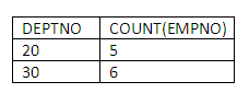
Figure 4.3
Comments: Department number 10 has four employees in our sample data set, and has been excluded from the results through the use of the HAVING clause.
The properties that are tested in a HAVING clause must be properties of groups, i.e. one must either test against individual values of the grouped-by item, such as:
HAVING JOB = ‘SALESMAN’
OR
JOB = ‘ANALYST’
or test against some property of the group, i.e. the number of members in the group (as in the example to exclude departments with less than five employees, or, for instance, tests on aggregate functions of the group - for our data set these could be properties such as the average or total salaries within the individual groups).
The HAVING clause, when required, always follows immediately after the GROUP BY clause to which it refers. It can contain compound conditions, linked by the boolean operators AND or OR (as above), and parentheses may be used to nest conditions.
It is not usually very long before a requirement arises to combine information from more than one table, into one coherent query result. For example, using the EMP and DEPT tables, we may wish to display the details of employee numbers and names, alongside the name of the department in which employees work. To do this, we will need to combine information from both the tables, as the employee details are stored in the EMP table, while the department name information is stored in the DEPT table (in the DNAME attribute).
The first point to note, is that this will mean listing both the EMP and DEPT tables in the table-list, following the FROM keyword in the query. In general, the table-list will contain all of the tables required to be accessed during the execution of a query. So far, as our queries have only ever accessed one table, the table-list has contained only one table. To list employee numbers and names with department names, however, the FROM clause will read:
FROM EMP, DEPT
Note that from a purely logical point of view, the order in which the tables are listed after the keyword FROM does not matter at all. In practice, however, if we are dealing with larger tables, the order of tables in the table-list may make a difference to the speed of execution of the query, as it may affect the order in which data from the tables is loaded into main memory from disk. This will be discussed further in the chapter on Advanced SQL.
Listing both the EMP and the DEPT tables after the FROM keyword, however, is not sufficient to achieve the results we are seeking. We don’t merely wish for the tables to be accessed in the query; we want the way in which they are accessed to be coordinated in a particular way. We wish to relate the display of a department name with the display of employee numbers and names of employees who work in that department. So we require the query to relate employee records in the EMP table with their corresponding department records in the DEPT table. The way this is achieved in SQL is by the Relational operator JOIN. The JOIN is an absolutely central concept in Relational databases, and therefore in the SQL language. It is such a central concept because this logical combining or relating of data from different tables is a common and important requirement in almost all applications. The ability to relate information from different tables in a uniform manner has been an important factor in the widespread adoption of Relational database systems.
A curious feature of performing JOINs, or relating information from different tables in a logical way as required in the above query, is that although the process is universally referred to as performing a JOIN, the way it is expressed in SQL does not always involve the use of the word JOIN. This can be particularly confusing for newcomers to JOINs. For example, to satisfy the query above, we would code the WHERE clause as follows:
WHERE EMP.DEPTNO = DEPT.DEPTNO
What this is expressing is that we wish rows in the EMP table to be related to rows in the DEPT table, by matching rows from the two tables whose department numbers (DEPTNOs) are equal. So we are using the DEPTNO column from each employee record in the EMP table, to link that employee record with the department record for that employee in the DEPT table.
The full query would therefore be:
SELECT EMPNO,ENAME,DNAME
FROM EMP,DEPT
WHERE EMP.DEPTNO = DEPT.DEPTNO;
This gives the following results for our test data set:
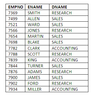
Figure 4.4
A few further points should be noted about the expression of the above query:
Because we wish to display values of the DNAME attribute in the result, it has, of course, to be included in the select-list.
We need not include any mention of the DEPTNO attribute in the select-list. We require the EMP.DEPTNO and DEPT.DEPTNO columns to perform the JOIN, so we refer to these columns in the WHERE clause, but we do not wish to display any DEPTNO information, therefore it is not included in the select-list.
As mentioned above, the order in which the EMP and DEPT tables appear after the FROM keyword is unimportant, at least assuming we can ignore issues of performance response, which we certainly can for tables of this size.
Similarly, the order in which the columns involved in the JOIN operation are expressed in the WHERE clause is also unimportant.
Example on joining two tables
List the names and jobs of employees, together with the locations in which they work:
SELECT ENAME,JOB,LOC
FROM EMP,DEPT
WHERE EMP.DEPTNO = DEPT.DEPTNO;
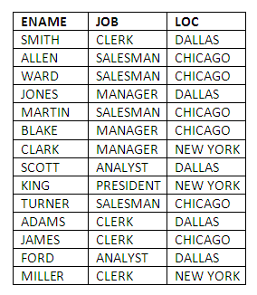
Figure 4.5
Comments: The exercise requires a simple modification to our first JOIN example – replacing EMPNO and DNAME in the select-list with the JOB and LOC attributes. LOC, like DNAME, is stored in the DEPT table, and so requires the coordination provided by a JOIN, in order to display employee information along with the locations of the departments in which those employees work.
The SQL standard provides the following alternative ways to specify this join:
FROM EMP JOIN DEPT ON EMP.DEPTNO = DEPT.DEPTNO;
FROM EMP JOIN DEPT USING DEPTNO;
FROM EMP NATURAL JOIN DEPT;
In each case, the FROM clause replaces the original FROM and WHERE clauses.
DEPTNO has been used as the data item to link records in the EMP and DEPT tables in the above examples. For our EMP and DEPT data set, DEPTNO is in fact the only semantically sensible possibility for use as the JOIN column. In the DEPT table, DEPTNO acts as the primary key (and as such must have a different value in every row within the DEPT table), while in the EMP table, DEPTNO acts as a foreign key, linking each EMP record with the department record in the DEPT table to which the employee record belongs. If we wish to refer to DEPTNO in the select-list, we would need to be careful to specify which instance of DEPTNO we are referring to: the one in the EMP table, or the one in the DEPT table. Failure to do this will lead to an error message indicating that the system is unable to identify which column we are referencing. The way to be specific about which instance of DEPTNO we require is simply to prefix the reference to the DEPTNO column with the table name containing that DEPTNO instance, placing a full stop (.) character between the table name and column name: for example, EMP.DEPTNO, or DEPT.DEPTNO. In this way, the system can identify which instance of DEPTNO is being referenced.
In general, if there is any possible ambiguity about which column is being referenced in a query, because a column with that name appears in more than one table, we use the table prefixing approach to clarify the reference. Note that this was not necessary when referencing any of the columns in the example JOIN queries above, as all of these appeared only once within either the EMP table or the DEPT table.
In addition to the basic form of the JOIN, also called a NATURAL JOIN and used to relate rows in different tables, we sometimes require a little more syntax than we have seen so far, in order to obtain all the information we require. Supposing, for example, we wish to list all departments with the employee numbers and names of their employees, plus any departments that do not contain employees.
As a first attempt, we might code:
SELECT DEPT.DEPTNO,DNAME,EMPNO,ENAME
FROM EMP,DEPT
WHERE EMP.DEPTNO = DEPT.DEPTNO
ORDER BY DEPT.DEPTNO;
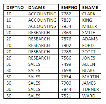
Figure 4.6
Comments: Note the use of DEPT.DEPTNO to specify the instance of the JOIN column unambiguously in the select-list. The ORDER BY clause is helpful in sorting the results into DEPT.DEPTNO order. In fact, ordering by DEPTNO, EMPNO would have been even more helpful, particularly in a larger data set. Incidentally, being clear which instance of DEPTNO we are referring to is just as important in the ORDER BY clause as it is in the select-list.
The results of this first attempt are, however, not the complete answer to the original query. Department number 40, called Operations, has no employees currently assigned to it, but it does not appear in the results.
The problem here is that the basic form of the JOIN only extracts matching instances of records from the joined tables. We need something further to force in any record instances that do not match a record in the other table. To do this, we use a construct called an OUTER JOIN. OUTER JOINs are used precisely in situations where we wish to force into our results set, rows that do and do not match a usual JOIN condition. There are three types of OUTER JOIN: LEFT, RIGHT, and FULL OUTER JOINS. To demonstrate the OUTER JOINs, we will use the following tables.
Person table
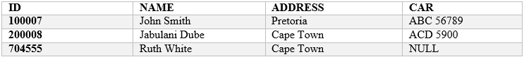
Figure 4.7
The person table holds the information of people. The ID is the primary key. A person can own a car or not.
Car table
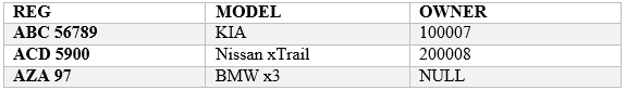
Figure 4.8
The car table holds information of cars. The REG is the primary key. A car can have an owner or not.
The syntax of the LEFT OUTER JOIN involves including the LEFT JOIN keyword in the query. Here's an example: List all persons together with their car’s registration and model, including any person without any car. The requirement is to force into the result set any person that does not have a car. To satisfy the requirement, we would write our query as such:
SELECT ID,NAME,REG,MODEL
FROM Person LEFT JOIN car ON Person.ID = Car.OWNER;
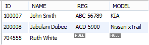
Figure 4.9
Comment: The query returns all the persons with cars, plus the one instance of a person (ID 704555) having no car.
Like a LEFT JOIN, the syntax of the RIGHT OUTER JOIN involves including the RIGHT JOIN keyword in the query. An example would be: List all cars together with their owner’s identification and name, including any car not owned by anyone.
SELECT REG,MODEL,ID,NAME
FROM Person RIGHT JOIN car ON Person.ID = Car.OWNER;
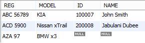
Figure 4.10
Comment: The query returns all the cars that are owned, plus the one instance of a car not owned by anyone.
If you wish to show both person records of those that don't own any car and car records that don't have any owner, then you need to use the FULL OUTER JOIN:
SELECT REG,MODEL,ID,NAME
FROM Person FULL JOIN car ON Person.ID = Car.OWNER;
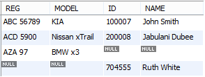
Figure 4.11
Table aliasing involves specifying aliases, or alternative names, that can be used to refer to the table during the processing of a query. The table aliases are specified in the table-list, following the FROM keyword. For example, the above FULL OUTER JOIN query can be written using aliases:
SELECT REG,MODEL,ID,NAME
FROM Person p FULL JOIN car c ON p.ID = c.OWNER;
Sometimes it is necessary to JOIN a table to itself in order to compare records from the same table. An example of this might be if we wish to compare values of salary on an individual basis between employees.
Example: find all employees who are paid more than “JONES”
What is required here is to compare the salaries of employees with the salary paid to JONES. A way of doing this, involves JOINing the EMP table with itself, so that we can carry out salary comparisons in the WHERE clause of an SQL query. However, if we wish to JOIN a table to itself, we need a mechanism for referring to the different rows being compared.
In order to specify the query to find out which employees are paid more than JONES, we shall use two table aliases, X and Y for the EMP table. We shall use X to denote employees whom we are comparing with JONES, and Y to denote JONES’ record specifically. This leads to the following query specification:
SELECT X.EMPNO,X.ENAME,X.SAL,Y.EMPNO,Y.ENAME,Y.SAL
FROM EMP X,EMP Y
WHERE X.SAL > Y.SAL
AND Y.ENAME = ‘JONES’
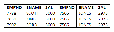
Figure 4.12
Comments: Note the use of the aliases for each of the column specifications in the select-list. We ensure that the alias Y is associated with the employee JONES through the second condition in the WHERE clause, “AND Y.ENAME = ‘JONES’”. The first condition in the WHERE clause, comparing salaries, ensures that apart from JONES’ record, which is listed in the result as a check on the query results, only the details of employees who are paid more than JONES are retrieved.
We have seen three forms of the JOIN condition. The basic JOIN, also called a NATURAL JOIN, is used to combine or coordinate the results of a query in a logical way across more than one table. In our examples, we have seen that JOINing two tables together involves one JOIN condition and, in general, JOINing N tables together requires the specification of N-1 JOIN conditions. A lot of work has gone into the development of efficient algorithms for the execution of JOINs in all the major database systems, with the result being that the overall performance of Relational database systems has seen a very considerable improvement since their introduction in the early '80s. In spite of this, JOINs are still an expensive operation in terms of query processing, and there can be situations where we seek ways of reducing the number of JOINs required to perform specific transactions.
Two further variants we have seen on the basic JOIN operation are the OUTER JOIN and the SELF JOIN. The OUTER JOIN is used to force non-matching records from one side of a JOIN into the set of retrieved results. The SELF JOIN is used where it is required to compare rows in a table with other rows from the same table. This comparison is facilitated through the use of aliases, alternative names which are associated with the table, and so can be used to reference the table on different sides of a JOIN specification.
The power of the SQL language is increased considerably through the ability to include one query within another. This is known as nesting queries, or writing sub-queries.
Nested query example
Find all employees who are paid more than JONES:
This might be considered a two-stage task:
Find Jones’ salary.
Find all those employees who are paid more than the salary found in step 1.
We might code step 1 as follows:
SELECT SAL
FROM EMP
WHERE ENAME = ‘JONES’
The nested query mechanism allows us to enclose this query within another one, which we might use to perform step 2:
SELECT EMPNO,ENAME,SAL
FROM EMP
WHERE SAL > …..
We simply need the syntax to enclose the query to implement step 1 in such a way that is provides its result to the query which implements step 2.
This is done by enclosing the query for step 1 in parentheses, and linking it to the query for step 2 as follows:
SELECT EMPNO,ENAME,SAL
FROM EMP
WHERE SAL >
(SELECT SAL FROM EMP WHERE ENAME = ‘JONES’);
This gives the following results:
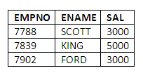
Figure 4.13
These are indeed the employees who earn more than JONES (who earns 2975).
Whenever a query appears to fall into a succession of natural steps such as the one above, it is a likely candidate to be coded as a nested query.
An important point has to be kept in mind when testing for equality of values across inner and outer queries.
If the inner query returns just one value, then we can use the equal sign, e.g.
SELECT …. FROM ….
WHERE ATTRIBUTE 1 = (SELECT ….
FROM …..)
If, however, the inner query might return more than one row, we must use the keyword IN, so that we can check whether the value of the attribute being tested in the WHERE clause of the outer query is IN the set of values returned by the inner query. Sub-queries can be included linked to a HAVING clause, i.e. they can retrieve a result which forms part of the condition in the evaluation of a HAVING clause. In this situation the format of the HAVING clause is:
HAVING ….
(SELECT … FROM .. WHERE ….)
The inner query may of course itself have inner queries, with WHERE, GROUP BY and HAVING clauses.
The number of queries that can be nested varies from one database system to another, but there is support for this SQL construct in all the leading databases such that there is no practical limit to the number of queries that can be nested.
In a similar way, a number of queries can be included at the same level of nesting, their results being combined together using the AND or OR keywords, according to the following syntax:
SELECT …. FROM ….
WHERE CONDITION 1 (SELECT ….
FROM ….. WHERE …..)
AND/OR (SELECT ….. FROM …. WHERE ….)
AND/OR
……
To find the details of any employees receiving the same salaries as either SCOTT or WARD, we could code:
SELECT EMPNO,ENAME,SAL
FROM EMP
WHERE SAL IN
(SELECT SAL FROM EMP
WHERE ENAME = ‘WARD’
OR
ENAME = ‘SCOTT’);
But suppose SCOTT and WARD are in different tables. If this is the case, we need to use the UNION operator in order to combine the results of queries on two different tables as follows:
SELECT EMPNO,ENAME,SAL
FROM EMP
WHERE SAL IN
(SELECT SAL
FROM EMP1
WHERE ENAME = ‘WARD’
UNION
SELECT SAL
FROM EMP2
WHERE ENAME = ‘SCOTT’);
Comments: We are assuming here that WARD is in a table called EMP1, and SCOTT in EMP2. The two salary values retrieved from these sub-queries are combined into a single results set, which is retrieved for comparison with all salary values in the EMP table in the outer query. Because there is more than one salary returned from the combined inner query, the IN keyword is used to make the comparison. Note that as with the Relational Algebra equivalent, the results of the SQL UNION operator must be union compatible, as we see they are in this case, as they both return single salary columns.
Again, like its Relational Algebra equivalent, the SQL INTERSECT operator can be used to extract the rows in common between two sets of query results:
SELECT JOB
FROM EMP
WHERE SAL > 2000 INTERSECT
SELECT JOB
FROM SHOPFLOORDETAILS;
Here the INTERSECT operator is used to find all jobs in common between the two queries. The first query returns all jobs that are paid more than 2000, whereas the second returns all jobs from a separate table called SHOPFLOORDETAILS. The final result, therefore, will be a list of all jobs in the SHOPFLOORDETAILS table that are paid more than 2000. Again, note that the sets of results compared with one another using the INTERSECT operator must be union compatible.
MINUS is used, like the DIFFERENCE operator of Relational Algebra, to subtract one set of results from another, where those results are derived from different tables.
For example:
SELECT EMPNO,ENAME,SAL
FROM EMP
WHERE ENAME IN
(SELECT ENAME
FROM EMP1
MINUS
SELECT ENAME
FROM EMP2);
Comments: The result of this query lists the details for employees whose names are the same as employees in table EMP1, with the exception of any names that are the same as employees in table EMP2.
The ANY or ALL operators may be used for sub-queries that return more than one row. They are used on the WHERE or HAVING clause in conjunction with the logical operators (=, !=, >, >=, <=, <). ANY compares a value to each value returned by a sub-query.
To display employees who earn more than the lowest salary in Department 30, enter:
SELECT ENAME, SAL, JOB, DEPTNO
FROM EMP
WHERE SAL >>
ANY
(SELECT DISTINCT SAL
FROM EMP
WHERE DEPTNO = 30)
ORDER BY SAL DESC;
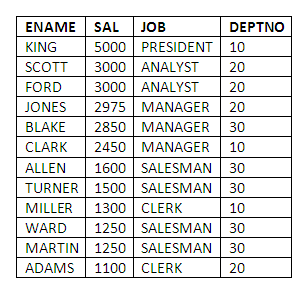
Figure 4.14
Comments: Note the use of the double >> sign, which is the syntax used in conjunction with the ANY and ALL operators to denote the fact that the comparison is carried out repeatedly during query execution. “= ANY” is equivalent to the keyword IN. With ANY, the DISTINCT keyword is often used in the sub-query to avoid the same values being selected several times. Clearly the lowest salary in department 30 is below 1100.
ALL compares a value to every value returned by a sub-query.
The following query finds employees who earn more than every employee in Department 30:
SELECT ENAME, SAL, JOB, DEPTNO
FROM EMP
WHERE SAL >>ALL
(SELECT DISTINCT SAL
FROM EMP
WHERE DEPTNO = 30)
ORDER BY SAL DESC;
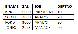
Figure 4.15
Comments: The inner query retrieves the salaries for Department 30. The outer query, using the All keyword, ensures that the salaries retrieved are higher than all of those in department 30. Clearly the highest salary in department 30 is below 2975.
Note that the NOT operator can be used with IN, ANY or ALL.
A correlated sub-query is a nested sub-query that is executed once for each 'candidate row' considered by the main query, and which on execution uses a value from a column in the outer query. This causes the correlated sub-query to be processed in a different way from the ordinary nested sub-query.
With a normal nested sub-query, the inner select runs first and it executes once, returning values to be used by the main query. A correlated sub-query, on the other hand, executes once for each candidate row to be considered by the outer query. The inner query is driven by the outer query.
Steps to execute a correlated sub-query:
The outer query fetches a candidate row.
The inner query is executed, using the value from the candidate row fetched by the outer query.
Whether the candidate row is retained depends on the values returned by the execution of the inner query.
Repeat until no candidate row remains.
Example
We can use a correlated sub-query to find employees who earn a salary greater than the average salary for their department:
SELECT EMPNO,ENAME,SAL,DEPTNO
FROM EMP E
WHERE SAL >> (SELECT AVG(SAL)
FROM EMP
WHERE DEPTNO = E.DEPTNO)
ORDER BY DEPTNO;
Giving the results:
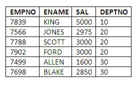
Figure 4.16
Comments: We can see immediately that this is a correlated sub-query since we have used a column from the outer select in the WHERE clause of the inner select. Note that the alias is necessary only to avoid ambiguity in column names.
A very useful facility is provided to enable users to run the same query again, entering a different value of a parameter to a WHERE or HAVING clause. This is done by prefixing the column specification for which different values are to be supplied by the “&” sign.
Example
Find the number of clerks based in department 10. Find the number of clerks in other departments by running the same query, in each case entering the value of the department number interactively.
SELECT COUNT(EMPNO) "NUMBER OF CLERKS"
FROM EMP
WHERE JOB = 'CLERK'
AND DEPTNO = &DEPTNO
The user will be asked to enter a value for DEPTNO. The result for entering 10 is:
Figure 4.17
This syntax provides a limited amount of interactivity with SQL queries, which can avoid the need to recode in order to vary the values of interactively specified parameters.
The following individual activities will provide practice by focusing on specific SQL constructs in each activity. These will be supplemented by the succeeding review questions, which will draw on all of the SQL material covered in this and the introductory chapter to SQL. This first activity will concentrate on various types of SQL JOIN.
Find all employees located in Dallas.
List the total annual pay for the Sales department (remember salary and commission data are provided as monthly figures).
List any departments that do not contain any employees.
Which workers earn more than their managers (hint: remember that the MGR attribute stores the EMPNO of an employee’s manager).
List the total monthly pay for each department.
List the number of employees located in Chicago and New York.
Find all jobs with more than two employees.
List the details of the highest-paid employee.
Find whether anyone in department 30 has the same job as JONES.
Find the job with the most employees.
Why is the JOIN operation such a core concept in Relational database systems? Describe how JOINs are expressed in SQL.
How can we express in SQL where it is required to JOIN more than two tables together?
Differentiate between the terms SELF JOIN and OUTER JOIN, and give a practical example of the use of each (you need not necessarily restrict yourself to the use of the data tables used in earlier examples).
Describe the use of the GROUP BY clause for categorising data in SQL.
What restrictions exist on the contents of a select-list which appears in the same query as a GROUP BY clause?
It is sometimes said that the HAVING keyword relates to the GROUP BY clause, in the same way that the WHERE keyword relates to SELECT. Explain the meaning of this statement, and draw parallels between the SELECT….WHERE and the GROUP BY …. HAVING constructs in SQL.
Describe the use of nested queries within the SQL language.
JOINs versus nested queries
In general, Relational database systems are optimised to perform JOIN operations very efficiently. It is also true that many SQL queries can be expressed either as a JOIN or as a nested query. Consider for yourself, and discuss online with colleagues, which of these two constructs you find easier to understand and to code. Do you find that any previous programming experience you may have had influences your ease of understanding and application of these concepts? For example, most people who have experience of conventional programming languages are familiar with loop statements and nesting one loop inside another, a construct which is very similar to a nested query. In general, do you think having had previous experience is an advantage or disadvantage when learning a language such as SQL?
Following on from the Additional Content section of the introductory chapter to SQL, you are encouraged to explore further the SQL support provided within Microsoft Access, or some other database of your choice, for the SQL constructs we have covered in this chapter.
Whereas you will have found relatively consistent support for all of the SQL features covered in the introductory chapter, now that we have covered the majority of the constructs available within the DML part of SQL, you are much more likely to find variations in support for the different features. These variations are likely to include:
Complete lack of support for some of the constructs covered, e.g. some databases do not allow nested queries at all, or do not support JOINs.
Partial support for some constructs; for example, some systems support nested queries, but do not support the keywords ANY and ALL.
Variations in the limits to how different constructs can be used; for example, some databases only allow query nesting to two or three levels, or support conventional JOINs but not the SELF or OUTER JOIN.
Using the sample tables provided in the database you have chosen, investigate the use of the SQL constructs described in this chapter, noting down differences and limitations in their implementation between your chosen database and the Oracle implementation.