Figure 11.1
Table of contents
At the end of this chapter you should be able to:
Describe how files and records can be placed on disks, and the effective ways in which records can be organised in files.
Describe a number of different types of indexes commonly found in modern database environments.
Understand the data structures which can support the various indexes.
Be fully aware of the proper ways in which indexes are used.
Use standard SQL syntax to create and remove different types of index on a set of tables.
Be aware of the typical approaches used in industry and commerce to improve database performance through indexing.
In parallel with this chapter, you should read Chapter 16 and Chapter 17 of Ramez Elmasri and Shamkant B. Navathe, " FUNDAMENTALS OF Database Systems", (7th edn.).
In this chapter, we will study how files and records can be placed on disks, and what the effective ways are in which records can be organised in files. The three file organisations we will learn in this chapter are heap file, sorted file and hash file. The only one goal in applying these various file organisation techniques is to provide the database system with good performance.
It is not only important that a database is designed well, but part of the design process also involves ensuring that the structure of the developed system is efficient enough to satisfy users’ requirements now and into the future.
Database tuning involves techniques that can be used to improve performance. It is an important and complex subject to which a number of chapters are devoted in this module. We will be looking into design issues of indexes, and the appropriate ways of using indexes. Indexes play a similar role in database systems as they do in books, in that they are used to speed up access to information. File structures can be affected by different indexing techniques, and they in turn will affect the performance of the databases.
It is worth emphasising again the importance of file organisations and their related access methods. Tuning techniques can help improve performance, but only to the extent that is allowed by a particular file organisation. For example, if you have a Ford car, you may obtain a better performance if you have the car’s engine tuned. However, no matter how hard you tune it, you will never be able to get a Ferrari’s performance out of it.
Indexes can help database developers build efficient file structures and offer effective access methods. When properly used and tuned, the database performance can be improved further. In fact, indexes are probably the single most important mechanism explicitly available to database developers and administrators for tuning the performance of a database.
The contents of this chapter are related to discussions on Database Administration and Further Performance Tuning Techniques.
In this chapter, we will describe the techniques used to store large amounts of structured data on disks. These techniques are important for database designers, DBAs (database administrators) and implementers of a DBMS. Database designers and DBAs must know the advantages and disadvantages of each storage method in order to develop and operate a DBMS for a specific application. Even an off-the-shelf DBMS will usually have different options available for organising the data, and the process of physical database design involves selecting the most appropriate data organisation technique for the given set of application requirements.
A typical database application will always need to access the database and retrieve some data for processing. Whenever a certain portion of the data is needed, it must be located on disk, loaded to main memory for processing, and then written back to the disk if changes have been made.
The data stored on disk is organised as files of records. Each record is a collection of data values that can be interpreted as facts about entities, their attributes and relationships. Records should be stored on disk in a manner that makes it possible to locate them efficiently whenever they are needed.
There are a number of commonly used file organisations which can determine how the records of a file are physically placed on disk. In this chapter, we will be discussing:
Heap file: which places records on disk in no particular order.
Sorted sequential file: which holds records in a particular order based on the value of a specified field (i.e. attribute).
Hashed file: which uses a hash function to decide where a record should be placed on disk.
In this chapter, we will also introduce access structures called indexes, which are used to speed up the retrieval of records if certain requirements on search conditions are met. An index for a file of records works just like an index catalogue in a library. In a normal library environment, for example, there should be catalogues such as author indexes and book title indexes. A user may use one of these indexes to quickly find the location of a required book, if he/she knows the author(s) or title of the book.
Each index (access structure) offers an access path to records. Some types of indexes, called secondary access paths, do not affect the physical placement of records on disk; rather, they provide alternative search paths for locating the records efficiently based on the indexing fields. Other types of indexes can only be constructed on a file with a particular primary organisation.
The focus of our study in this chapter will be on the following:
Primary indexes
Clustering indexes
Secondary indexes
Multilevel indexes
B-tree and B+ tree structures.
It must be emphasised that different indexes have their own advantages and disadvantages. There is no universally efficient index. Each technique is best suited for a particular type of database application.
The merits of indexes can be measured in the following aspects:
Access types: The kind of access methods that can be supported efficiently (e.g. value-based search or range search).
Access time: Time needed to locate a particular record or a set of records.
Insertion efficiency: How efficient an insertion operation is.
Deletion efficiency: How efficient a deletion operation is.
Storage overhead: The additional storage requirement of an index structure.
It is worth noting that a file of records can have more than one index, just like for books there can be different indexes such as author index and title index.
An index access structure is usually constructed on a single field of a record in a file, called an indexing field. Such an index typically stores each value of the indexing field, along with a list of pointers to all disk blocks that contain records with that field value. The values in the index are usually sorted (ordered) so that we can perform an efficient binary search on the index.
To give you an intuitive understanding of an index, we look at library indexes again. For example, an author index in a library will have entries for all authors whose books are stored in the library. AUTHOR is the indexing field and all the names are sorted according to alphabetical order. For a particular author, the index entry will contain locations (i.e. pointers) of all the books this author has written. If you know the name of the author, you will be able to use this index to find his/her books quickly. What happens if you do not have an index to use? This is similar to using a heap file and linear search. You will have to browse through the whole library looking for the book.
An index file is much smaller than the data file, and therefore searching the index using a binary search can be carried out quickly. Multilevel indexing goes one step further in the sense that it eliminates the need for a binary search, by building indexes to the index itself. We will be discussing these techniques later on in the chapter.
In this section, we will briefly define the concepts of records, record types and files. Then we will discuss various techniques for organising file records on disk.
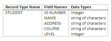
A record is a unit which data is usually stored in. Each record is a collection of related data items, where each item is formed of one or more bytes and corresponds to a particular field of the record. Records usually describe entities and their attributes. A collection of field (item) names and their corresponding data types constitutes a record type. In short, we may say that a record type corresponds to an entity type and a record of a specific type represents an instance of the corresponding entity type.
The following is an example of a record type and its record:
Figure 11.1
A specific record of the STUDENT type:
STUDENT(9901536, "James Bond", "1 Bond Street, London", "Intelligent Services", 9)
A file basically contains a sequence of records. Usually all records in a file are of the same record type. If every record in the file has the same size in bytes, the records are called fixed-length records. If records in the file have different sizes, they are called variable-length records.
Variable-length records may exist in a file for the following reasons:
Although they may be of the same type, one or more of the fields may be of varying length. For instance, students’ names are of different lengths.
The records are of the same type, but one or more of the fields may be a repeating field with multiple values.
If one or more fields are optional, not all records (of the same type) will have values for them.
A file may contain records of different record types. In this case, records in the file are likely to have different sizes.
For fixed-length records, the exact size of each record can be determined in advance. As a result, they can easily be allocated to blocks (a block is the unit of transfer of data between main memory and disk). Also, we can identify the starting byte position of each field relative to the starting position of the record, because each of such records has the same fields, and the field lengths are fixed and known beforehand. This provides us with a simple way to find field values of a record in the file.
For records with variable-length fields, we may not know the exact lengths of those fields in advance. In order to determine the bytes that are needed to accommodate those fields, we can use special separator characters, which do not appear in any field value (such as ~, @, or !), to terminate the variable-length fields. An alternative to this approach is to store the exact length of a variable-length field explicitly in the record concerned.
A repeating field needs one separator character to separate the repeating values of the field, and another separator character to indicate termination of the field. In short, we need to find out the exact size of a variable-length record before allocating it to a block or blocks. It is also apparent that programs that process files of variable-length records will be more complex than those for fixed-length records, where the starting position and size of each field are known and fixed.
We have seen that fixed-length records have advantages over variable-length records with respect to storage and retrieving a field value within the record. In some cases, therefore, it is possible and may also be advantageous to use a fixed-length record structure to represent a record that may logically be of variable length.
For example, we can use a fixed-length record structure that is large enough to accommodate the largest variable-length record anticipated in the file. For a repeating field, we could allocate as many spaces in each record as the maximum number of values that the field can take. In the case of optional fields, we may have every field included in every file record. If an optional field is not applicable to a certain record, a special null value is stored in the field. By adopting such an approach, however, it is likely that a large amount of space will be wasted in exchange for easier storage and retrieval.
The records of a file must be allocated to disk blocks because a block is the unit of data transfer between disk and main memory. When the record size is smaller than the block size, a block can accommodate many such records. If a record has too large a size to be fitted in one block, two or more blocks will have to be used.
In order to enable further discussions, suppose the size of the block is B bytes, and a file contains fixed-length records of size R bytes. If B # R, then we can allocate bfr = #(B/R)# records into one block, where #(x)# is the so-called floor function which rounds the value x down to the next integer. The value bfr is defined as the blocking factor for the file.
In general, R may not divide B exactly, so there will be some leftover spaces in each block equal to B – (bfr * R) bytes .
If we do not want to waste the unused spaces in the blocks, we may choose to store part of a record in them and the rest of the record in another block. A pointer at the end of the first block points to the block containing the other part of the record, in case it is not the next consecutive block on disk. This organisation is called 'spanned', because records can span more than one block. If records are not allowed to cross block boundaries, the organisation is called 'unspanned'.
Unspanned organisation is useful for fixed-length records with a length R # B. It makes each record start at a known location in the block, simplifying record processing. For variable-length records, either a spanned or unspanned organisation can be used. It is normally advantageous to use spanning to reduce the wasted space in each block.
For variable-length records using spanned organisation, each block may store a different number of records. In this case, the blocking factor bfr represents the average number of records per block for the file. We can then use bfr to calculate the number of blocks (b) needed to accommodate a file of r records:
b = #(r/bfr)# blocks
where #(x)# is the so-called ceiling function which rounds the value x up to the nearest integer.
It is not difficult to see that if the record size R is bigger than the block size B, then spanned organisation has to be used.
A file normally contains a file header or file descriptor providing information which is needed by programs that access the file records. The contents of a header contain information that can be used to determine the disk addresses of the file blocks, as well as to record format descriptions, which may include field lengths and order of fields within a record for fixed-length unspanned records, separator characters, and record type codes for variable-length records.
To search for a record on disk, one or more blocks are transferred into main memory buffers. Programs then search for the desired record or records within the buffers, using the header information.
If the address of the block that contains the desired record is not known, the programs have to carry out a linear search through the blocks. Each block is loaded into a buffer and checked until either the record is found or all the blocks have been searched unsuccessfully (which means the required record is not in the file). This can be very time-consuming for a large file. The goal of a good file organisation is to locate the block that contains a desired record with a minimum number of block transfers.
Operations on files can usually be grouped into retrieval operations and update operations. The former do not change anything in the file, but only locate certain records for further processing. The latter change the file by inserting or deleting or modifying some records.
Typically, a DBMS can issue requests to carry out the following operations (with assistance from the operating-system file/disk managers):
Find (or Locate): Searches for the first record satisfying a search condition (a condition specifying the criteria that the desired records must satisfy). Transfers the block containing that record into a buffer (if it is not already in main memory). The record is located in the buffer and becomes the current record (ready to be processed).
Read (or Get): Copies the current record from the buffer to a program variable. This command may also advance the current record pointer to the next record in the file.
FindNext: Searches for the next record in the file that satisfies the search condition. Transfers the block containing that record into a buffer, and the record becomes the current record.
Delete: Deletes the current record and updates the file on disk to reflect the change requested.
Modify: Modifies some field values for the current record and updates the file on disk to reflect the modification.
Insert: Inserts a new record in the file by locating the block where the record is to be inserted, transferring that block into a buffer, writing the (new) record into the buffer, and writing the buffer to the disk file to reflect the insertion.
FindAll: Locates all the records in the file that satisfy a search condition.
FindOrdered: Retrieves all the records in the file in a specified order.
Reorganise: Rearranges records in a file according to certain criteria. An example is the 'sort' operation, which organises records according to the values of specified field(s).
Open: Prepares a file for access by retrieving the file header and preparing buffers for subsequent file operations.
Close: Signals the end of using a file.
Before we move on, two concepts must be clarified:
File organisation: This concept generally refers to the organisation of data into records, blocks and access structures. It includes the way in which records and blocks are placed on disk and interlinked. Access structures are particularly important. They determine how records in a file are interlinked logically as well as physically, and therefore dictate what access methods may be used.
Access method: This consists of a set of programs that allow operations to be performed on a file. Some access methods can only be applied to files organised in certain ways. For example, indexed access methods can only be used in indexed files.
In the following sections, we are going to study three file organisations, namely heap files, sorted files and hash files, and their related access methods.
Review question 1
What are the different reasons for having variable-length records?
How can we determine the sizes of variable-length records with variable-length fields when allocating them to disk?
When is it most useful to use fixed-length representations for a variable-length record?
What information is stored in file headers?
What is the difference between a file organisation and an access method?
The heap file organisation is the simplest and most basic type of organisation. In such an organisation, records are stored in the file in the order in which they are inserted, and new records are always placed at the end of the file.
The insertion of a new record is very efficient. It is performed in the following steps:
The last disk block of the file is copied into a buffer.
The new record is added.
The block in the buffer is then rewritten back to the disk.
Remember the address of the last file block can always be kept in the file header.
The search for a record based on a search condition involves a linear search through the file block by block, which is often a very inefficient process. If only one record satisfies the condition then, on average, half of the file blocks will have to be transferred into main memory before the desired record is found. If no records or several records satisfy the search condition, all blocks will have to be transferred.
To modify a record in a file, a program must:
find it;
transfer the block containing the record into a buffer;
make the modifications in the buffer;
then rewrite the block back to the disk.
As we have seen, the process of finding the record can be time-consuming.
To remove a record from a file, a program must:
find it;
transfer the block containing the record into a buffer;
delete the record from the buffer;
then rewrite the block back to the disk.
Again, the process of finding the record can be time-consuming.
Physical deletion of a record leaves unused space in the block. As a consequence, a large amount of space may be wasted if frequent deletions have taken place. An alternative method to physically deleting a record is to use an extra bit (called a deletion marker) in all records. A record is deleted (logically) by setting the deletion marker to a particular value. A different value of the marker indicates a valid record (i.e. not deleted). Search programs will only consider valid records in a block. Invalid records will be ignored as if they have been physically removed.
No matter what deletion technique is used, a heap file will require regular reorganisation to reclaim the unused spaces due to record deletions. During such reorganisation, the file blocks are accessed consecutively and some records may need to be relocated to fill the unused spaces. An alternative approach to reorganisation is to use the space of deleted records when inserting new records. However, this alternative will require extra facilities to keep track of empty locations.
Both spanned and unspanned organisations can be used for a heap file of either fixed-length records or variable-length records. Modifying a variable-length record may require deleting the old record and inserting a new record incorporating the required changes, because the modified record may not fit in its old position on disk.
Exercise 1
A file has r = 20,000 STUDENT records of fixed length, each record has the following fields: ID# (7 bytes), NAME (35 bytes), ADDRESS (46 bytes), COURSE (12 bytes), and LEVEL (1 byte). An additional byte is used as a deletion marker. This file is stored on the disk with the following characteristics: block size B = 512 bytes; inter-block gap size G = 128 bytes; number of blocks per track = 20; number of tracks per surface = 400. Do the following exercises:
Calculate the record size R.
Calculate the blocking factor bfr.
Calculate the number of file blocks b needed to store the records, assuming an unspanned organisation.
Exercise 2
Suppose we now have a new disk device which has the following specifications: block size B = 2400 bytes; inter-block gap size G = 600 bytes. The STUDENT file in Exercise 1 is stored on this disk, using unspanned organisation. Do the following exercises:
Calculate the blocking factor bfr.
Calculate the wasted space in each disk block because of the unspanned organisation.
Calculate the number of file blocks b needed to store the records.
Calculate the average number of block accesses needed to search for an arbitrary record in the file, using linear search.
Review question 2
Discuss the different techniques for record deletion.
Records in a file can be physically ordered based on the values of one of their fields. Such a file organisation is called a sorted file, and the field used is called the ordering field. If the ordering field is also a key field, then it is called the ordering key for the file.
The following figure depicts a sorted file organisation containing the STUDENT records:
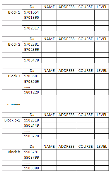
Figure 11.2
The sorted file organisation has some advantages over unordered files, such as:
Reading the records in order of the ordering field values becomes very efficient, because no sorting is required. (Remember, one of the common file operations is FindOrdered.)
Locating the next record from the current one in order of the ordering field usually requires no additional block accesses, because the next record is often stored in the same block (unless the current record is the last one in the block).
Retrieval using a search condition based on the value of the ordering field can be efficient when the binary search technique is used.
In general, the use of the ordering field is essential in obtaining the advantages.
A binary search for disk files can be performed on the blocks rather than on the records. Suppose that:
the file has b blocks numbered 1, 2, ..., b;
the records are ordered by ascending value of their ordering key;
we are searching for a record whose ordering field value is K;
disk addresses of the file blocks are available in the file header.
The search algorithm is described below in pseudo-codes:
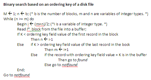
Figure 11.3
Explanations:
The binary search algorithm always begins from the middle block in the file. The middle block is loaded into a buffer.
Then the specified ordering key value K is compared with that of the first record and the last record in the buffer.
If K is smaller than the ordering field value of the first record, then it means that the desired record must be in the first half of the file (if it is in the file at all). In this case, a new binary search starts in the upper half of the file and blocks in the lower half can be ignored.
If K is bigger than the ordering field value of the last record, then it means that the desired record must be in the second half of the file (if it is in the file at all). In this case, a new binary search starts in the lower half of the file and blocks in the upper half can be ignored.
If K is between the ordering field values of the first and last records, then it should be in the block already in the buffer. If not, it means the record is not in the file at all.
Referring to the example in the figure above, suppose we want to find a student’s record whose ID number is 9701890. We further assume that there are five blocks in the file (i.e. the five blocks shown in the figure). Using the binary search, we start in block 3 and find that 9701890 (the specified ordering field value) is smaller than 9703501 (the ordering field value of the first record). Thus, we move to block 2 and read it into the buffer. Again, we find that 9701890 is smaller than 9702381 (the ordering field value of the first record of block 2). As a result, we read in block 1 and find 9701890 is between 9701654 and 9702317. If the record is in the file, it has to be in this block. By conducting a further search in the buffer, we can find the record.
The sorted file organisation can offer very efficient retrieval performance only if the search is based on the ordering field values. For example, the search for the following SQL query is efficient:
select NAME, ADDRESS from STUDENT
where ID# = 9701890;
If ID# is not in the condition, the linear search has to be used and there will be no performance advantages.
Update operations (e.g. insertion and deletion) are expensive for an ordered file because we must always maintain the order of records in the file.
To insert a new record, we must first find its correct position among existing records in the file, according to its ordering field value. Then a space has to be made at that location to store it. This involves reorganisation of the file, and for a large file it can be very time-consuming. The reason is that on average, half the records of the file must be moved to make the space. For record deletion, the problem is less severe, if deletion markers are used and the file is reorganised periodically.
One option for making insertion more efficient is to keep some unused space in each block for new records. However, once this space is used up, the original problem resurfaces.
The performance of a modification operation depends on two factors: first, the search condition to locate the record, and second, the field to be modified.
If the search condition involves the ordering field, the efficient binary search can be used. Otherwise, we have to conduct a linear search.
A non-ordering field value can be changed and the modified record can be rewritten back to its original location (assuming fixed-length records).
Modifying the ordering field value means that the record may change its position in the file, which requires the deletion of the old record followed by the insertion of the modified one as a new record.
Reading the file records in order of the ordering field is efficient. For example, the operations corresponding to the following SQL query can be performed efficiently:
select ID#, NAME, COURSE from STUDENT
where LEVEL = 2
order by ID#;
The sorted file organisation is rarely used in databases unless a primary index structure is included with the file. The index structure can further improve the random access time based on the ordering field.
Review question 3
What major advantages do sorted files have over heap files?
What is the essential element in taking full advantage of the sorted organisation?
Describe the major problems associated with the sorted files.
Exercise 3
Suppose we have the same disk and STUDENT file as in Exercise 2. This time, however, we assume that the records are ordered based on ID# in the disk file. Calculate the average number of block accesses needed to search for a record with a given ID#, using binary search.
The hash file organisation is based on the use of hashing techniques, which can provide very efficient access to records based on certain search conditions. The search condition must be an equality condition on a single field called hash field (e.g. ID# = 9701890, where ID# is the hash field). Often the hash field is also a key field. In this case, it is called the hash key.
The principle idea behind the hashing technique is to provide a function h, called a hash function, which is applied to the hash field value of a record and computes the address of the disk block in which the record is stored. A search for the record within the block can be carried out in a buffer, as always. For most records, we need only one block transfer to retrieve that record.
Suppose K is a hash key value, the hash function h will map this value to a block address in the following form:
h(K) = address of the block containing the record with the key value K
If a hash function operates on numeric values, then non-numeric values of the hash field will be transformed into numeric ones before the function is applied.
The following are two examples of many possible hash functions:
Hash function h(K) = K mod M: This function returns the remainder of an integer hash field value K after division by integer M. The result of the calculation is then used as the address of the block holding the record.
A different function may involve picking some digits from the hash field value (e.g. the 2nd, 4th and 6th digits from ID#) to form an integer, and then further calculations may be performed using the integer to generate the hash address.
The problem with most hashing functions is that they do not guarantee that distinct values will hash to distinct addresses. The reason is that the hash field space (the number of possible values a hash field can take) is usually much larger than the address space (the number of available addresses for records). For example, the hash function h(K) = K mod 7 will hash 15 and 43 to the same address 1 as shown below:
43 mod 7 = 1
15 mod 7 = 1
A collision occurs when the hash field value of a new record that is being inserted hashes to an address that already contains a different record. In this situation, we must insert the new record in some other position. The process of finding another position is called collision resolution.
The following are commonly used techniques for collision resolution:
Open addressing: If the required position is found occupied, the program will check the subsequent positions in turn until an available space is located.
Chaining: For this method, some spaces are kept in the disk file as overflow locations. In addition, a pointer field is added to each record location. A collision is resolved by placing the new record in an unused overflow location and setting the pointer of the occupied hash address location to the address of that overflow location. A linked list of overflow records for each hash address needs to be maintained.
Multiple hashing: If a hash function causes a collision, a second hash function is applied. If it still does not resolve the collision, we can then use open addressing or apply a third hash function and so on.
Each collision resolution method requires its own algorithms for insertion, retrieval, and deletion of records. Detailed discussions on them are beyond the scope of this chapter. Interested students are advised to refer to textbooks dealing with data structures.
In general, the goal of a good hash function is to distribute the records uniformly over the address space and minimise collisions, while not leaving many unused locations. Also remember that a hash function should not involve complicated computing. Otherwise, it may take a long time to produce a hash address, which will actually hinder performance.
Hashing for disk files is called external hashing. To suit the characteristics of disk storage, the hash address space is made of buckets. Each bucket consists of either one disk block or a cluster of contiguous (neighbouring) blocks, and can accommodate a certain number of records.
A hash function maps a key into a relative bucket number, rather than assigning an absolute block address to the bucket. A table maintained in the file header converts the relative bucket number into the corresponding disk block address.
The collision problem is less severe with buckets, because as many records as will fit in a bucket can hash to the same bucket without causing any problem. If the collision problem does occur when a bucket is filled to its capacity, we can use a variation of the chaining method to resolve it. In this situation, we maintain a pointer in each bucket to a linked list of overflow records for the bucket. The pointers in the linked list should be record pointers, which include both a block address and a relative record position within the block.
Some hashing techniques allow the hash function to be modified dynamically to accommodate the growth or shrinkage of the database. These are called dynamic hash functions.
Extendable hashing is one form of dynamic hashing, and it works in the following way:
We choose a hash function that is uniform and random. It generates values over a relatively large range.
The hash addresses in the address space (i.e. the range) are represented by d-bit binary integers (typically d = 32). As a result, we can have a maximum of 232 (over 4 billion) buckets.
We do not create 4 billion buckets at once. Instead, we create them on demand, depending on the size of the file. According to the actual number of buckets created, we use the corresponding number of bits to represent their address. For example, if there are four buckets at the moment, we just need 2 bits for the addresses (i.e. 00, 01, 10 and 11).
At any time, the actual number of bits used (denoted as i and called global depth) is between 0 (for one bucket) and d (for maximum 2d buckets).
Value of i grows or shrinks with the database, and the i binary bits are used as an offset into a table of bucket addresses (called a directory). In Figure 11.3, 3 bits are used as the offset (i.e. 000, 001, 010, ..., 110, 111).
The offsets serve as indexes pointing to the buckets in which the corresponding records are held. For example, if the first 3 bits of a hash value of a record are 001, then the record is in the bucket pointed by the 001 entry.
It must be noted that there does not have to be a distinct bucket for each of the 2i directory locations. Several directory locations (i.e. entries) with the same first j bits (j <= i) for their hash values may contain the same bucket address (i.e. point to the same bucket) if all the records that hash to these locations fit in a single bucket.
j is called the local depth stored with each bucket. It specifies the number of bits on which the bucket contents are based. In Figure 11.3, for example, the middle two buckets contain records which have been hashed based on the first 2 bits of their hash values (i.e. starting with 01 and 10), while the global depth is 3.
The value of i can be increased or decreased by one at a time, thus doubling or halving the number of entries in the directory table. Doubling is needed if a bucket whose local depth j is equal to the global depth i, overflows. Halving occurs if i > j for all the buckets after some deletions occur.
Retrieval - To find the bucket containing the search key value K:
Compute h(K).
Take the first i bits of h(K).
Look at the corresponding table entry for this i-bit string.
Follow the bucket pointer in the table entry to retrieve the block.
Insertion - To add a new record with the hash key value K:
Follow the same procedure for retrieval, ending up in some bucket.
If there is still space in that bucket, place the record in it.
If the bucket is full, we must split the bucket and redistribute the records.
If a bucket is split, we may need to increase the number of bits we use in the hash.
To illustrate bucket splitting (see the figure below), suppose that a new record to be inserted causes overflow in the bucket whose hash values start with 01 (the third bucket). The records in that bucket will have to be redistributed among two buckets: the first contains all records whose hash values start with 010, and the second contains all those whose hash values start with 011. Now the two directory entries for 010 and 011 point to the two new distinct buckets. Before the split, they point to the same bucket. The local depth of the two new buckets is 3, which is one more than the local depth of the old bucket.
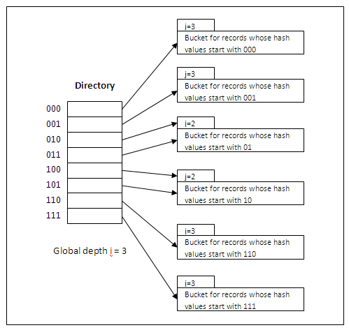
Figure 11.4
If a bucket that overflows and is split used to have a local depth j equal to the global depth i of the directory, then the size of the directory must now be doubled so that we can use an extra bit to distinguish the two new buckets. In the above figure, for example, if the bucket for records whose hash values start with 111 overflows, the two new buckets need a directory with global depth i = 4, because the two buckets are now labelled 1110 and 1111, and hence their local depths are both 4. The directory size is doubled and each of the other original entries in the directory is also split into two, both with the same pointer as the original entries.
Deletion may cause buckets to be merged and the bucket address directory may have to be halved.
In general, most record retrievals require two block accesses – one to the directory and the other to the bucket. Extendable hashing provides performance that does not degrade as the file grows. Space overhead is minimal, because no buckets need be reserved for future use. The bucket address directory only contains one pointer for each hash value of current prefix length (i.e. the global depth). Potential drawbacks are that we need to have an extra layer in the structure (i.e. the directory) and this adds more complexities.
Hashing provides the fastest possible access for retrieving a record based on its hash field value. However, search for a record where the hash field value is not available is as expensive as in the case of a heap file.
Record deletion can be implemented by removing the record from its bucket. If the bucket has an overflow chain, we can move one of the overflow records into the bucket to replace the deleted record. If the record to be deleted is already in the overflow, we simply remove it from the linked list.
To insert a new record, first, we use the hash function to find the address of the bucket the record should be in. Then, we insert the record into an available location in the bucket. If the bucket is full, we will place the record in one of the locations for overflow records.
The performance of a modification operation depends on two factors: first, the search condition to locate the record, and second, the field to be modified.
If the search condition is an equality comparison on the hash field, we can locate the record efficiently by using the hash function. Otherwise, we must perform a linear search.
A non-hash field value can be changed and the modified record can be rewritten back to its original bucket.
Modifying the hash field value means that the record may move to another bucket, which requires the deletion of the old record followed by the insertion of the modified one as a new record.
One of the most notable drawbacks of commonly used hashing techniques (as presented above) is that the amount of space allocated to a file is fixed. In other words, the number of buckets is fixed, and the hashing methods are referred to as static hashing. The following problems may occur:
The number of buckets is fixed, but the size of the database may grow.
If we create too many buckets, a large amount of space may be wasted.
If there are too few buckets, collisions will occur more often.
As the database grows over time, we have a few options:
Devise a hash function based on current file size. Performance degradation will occur as the file grows, because the number of buckets will appear to be too small.
Devise a hash function based on the expected file size. This may mean the creation of too many buckets initially and cause some space wastage.
Periodically reorganise the hash structure as file grows. This requires devising new hash functions, recomputing all addresses and generating new bucket assignments. This can be costly and may require the database to be shut down during the process.
Review question 4
What is a collision and why is it unavoidable in hashing?
How does one cope with collisions in hashing?
What are the most notable problems that static hashing techniques have?
Suppose we have a VIDEO file holding VIDEO_TAPE records for a rental shop. The records have TAPE# as the hash key with the following values: 2361, 3768, 4684, 4879, 5651, 1829, 1082, 7107, 1628, 2438, 3951, 4758, 6967, 4989, 9201. The file uses eight buckets, numbered 0 to 7. Each bucket is one disk block and can store up to two records. Load the above records into the file in the given order, using the hash function h(K) = K mod 8. The open addressing method is used to deal with any collision.
Show how the records are stored in the buckets.
Calculate the average number of block accesses needed for a random retrieval based on TAPE#.
Activity 1 - Record Deletion in Extensible Hashing
The purpose of this activity is to enable you to consolidate what you have learned about extendable hashing. You should work out yourself how to delete a record from a file with the extendable hashing structure. What happens if a bucket becomes empty due to the deletion of its last record? When the size of the directory may need to be halved?
There are several types of single-level ordered indexes. A primary index is an index specified on the ordering key field of a sorted file of records. If the records are sorted not on the key field but on a non-key field, an index can still be built that is called a clustering index. The difference lies in the fact that different records have different values in the key field, but for a non-key field, some records may share the same value. It must be noted that a file can have at most one physical ordering field. Thus, it can have at most one primary index or one clustering index, but not both.
A third type of index, called a secondary index, can be specified on any non-ordering field of a file. A file can have several secondary indexes in addition to its primary access path (i.e. primary index or clustering index). As we mentioned earlier, secondary indexes do not affect the physical organisation of records.
A primary index is built for a file (the data file) sorted on its key field, and itself is another sorted file (the index file) whose records (index records) are of fixed-length with two fields. The first field is of the same data type as the ordering key field of the data file, and the second field is a pointer to a disk block (i.e., the block address).
The ordering key field is called the primary key of the data file. There is one index entry (i.e., index record) in the index file for each block in the data file. Each index entry has the value of the primary key field for the first record in a block and a pointer to that block as its two field values. We use the following notation to refer to an index entry i in the index file:
<K(i), P(i)>
K(i) is the primary key value, and P(i) is the corresponding pointer (i.e. block address).
For example, to build a primary index on the sorted file shown below (this is the same STUDENT file we saw in exercise 1), we use the ID# as primary key, because that is the ordering key field of the data file:
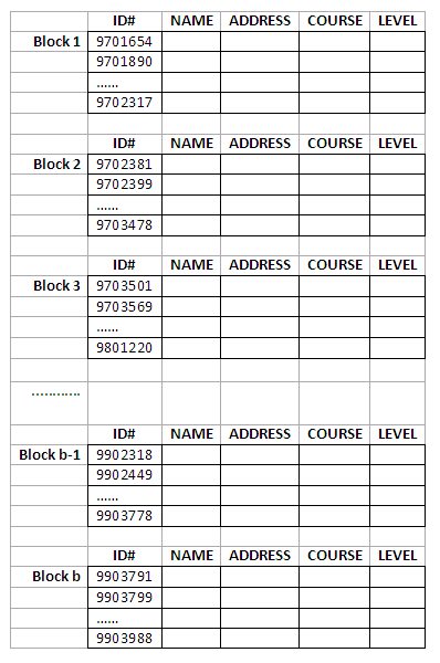
Figure 11.5
Each entry in the index has an ID# value and a pointer. The first three index entries of such an index file are as follows:
<K(1) = 9701654, P(1) = address of block 1>
<K(2) = 9702381, P(2) = address of block 2>
<K(3) = 9703501, P(3) = address of block 3>
The figure below depicts this primary index. The total number of entries in the index is the same as the number of disk blocks in the data file. In this example, there are b blocks.
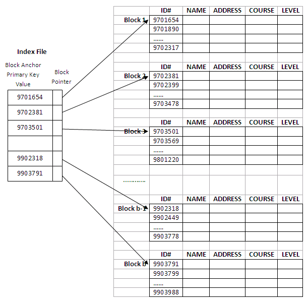
Figure 11.6
The first record in each block of the data file is called the anchor record of that block. A variation to such a primary index scheme is that we could use the last record of a block as the block anchor. However, the two schemes are very similar and there is no significant difference in performance. Thus, it is sufficient to discuss just one of them.
A primary index is an example of a sparse index, in the sense that it contains an entry for each disk block rather than for every record in the data file. A dense index, on the other hand, contains an entry for every data record. A dense index does not require the data file to be a sorted file. Instead, it can be built on any file organisation (typically, a heap file).
By definition, an index file is just a special type of data file of fixed-length records with two fields. We use the term 'index file' to refer to data files storing index entries. The general term 'data file' is used to refer to files containing the actual data records such as STUDENT.
The index file for a primary index needs significantly fewer blocks than does the file for data records for the following two reasons:
There are fewer index entries than there are records in the data file, because an entry exists for each block rather than for each record.
Each index entry is typically smaller in size than a data record because it has only two fields. Consequently, more index entries can fit into one block. A binary search on the index file hence requires fewer block accesses than a binary search on the data file.
If a record whose primary key value is K is in the data file, then it has to be in the block whose address is P(i), where K(i) <= K < K(i+1). The ith block in the data file contains all such records because of the physical ordering of the records based on the primary key field. For example, look at the first three entries in the index in the last figure.
<K(1) = 9701654, P(1) = address of block 1>
<K(2) = 9702381, P(2) = address of block 2>
<K(3) = 9703501, P(3) = address of block 3>
The record with ID#=9702399 is in the 2nd block because K(2) <= 9702399 < K(3). In fact, all the records with an ID# value between K(2) and K(3) must be in block 2, if they are in the data file at all.
To retrieve a record, given the value K of its primary key field, we do a binary search on the index file to find the appropriate index entry i, and then use the block address contained in the pointer P(i) to retrieve the data block. The following example explains the performance improvement, in terms of the number of block accesses that can be obtained through the use of primary index.
Example 1
Suppose that we have an ordered file with r = 40,000 records stored on a disk with block size B = 1024 bytes. File records are of fixed-length and are unspanned, with a record size R = 100 bytes. The blocking factor for the data file would be bfr = #(B/R)## = #(1024/100)## = 10 records per block. The number of blocks needed for this file is b = #(r/bfr)## = #(40000/10)## = 4000 blocks. A binary search on the data file would need approximately #(log2b)## = #(log24000)## = 12 block accesses.
Now suppose that the ordering key field of the file is V = 11 bytes long, a block pointer (block address) is P = 8 bytes long, and a primary index has been constructed for the file. The size of each index entry is Ri = (11 + 8) = 19 bytes, so the blocking factor for the index file is bfr i = #(B/Ri)## = #(1024/19)#
# = 53 entries per block. The total number of index entries ri is equal to the number of blocks in the data file, which is 4000. Thus, the number of blocks needed for the index file is bi = #(ri/bfri)### = #(4000/53)### = 76 blocks. To perform a binary search on the index file would need #(log2bi)### = #(log276)### = 7 block accesses. To search for the actual data record using the index, one additional block access is needed. In total, we need 7 + 1 = 8 block accesses, which is an improvement over binary search on the data file, which required 12 block accesses.
A major problem with a primary index is insertion and deletion of records. We have seen similar problems with sorted file organisations. However, they are more serious with the index structure because, if we attempt to insert a record in its correct position in the data file, we not only have to move records to make space for the newcomer but also have to change some index entries, since moving records may change some block anchors. Deletion of records causes similar problems in the other direction.
Since a primary index file is much smaller than the data file, storage overhead is not a serious problem.
Exercise 4
Consider a disk with block size B = 512 bytes. A block pointer is P = 8 bytes long, and a record pointer is Pr = 9 bytes long. A file has r = 50,000 STUDENT records of fixed-size R = 147 bytes. In the file, the key field is ID#, whose length V = 12 bytes. Answer the following questions:
If an unspanned organisation is used, what are the blocking factor bfr and the number of file blocks b?
Suppose that the file is ordered by the key field ID# and we want to construct a primary index on ID#. Calculate the index blocking factor bfri.
What are the number of first-level index entries and the number of first-level index blocks?
Determine the number of block accesses needed to search for and retrieve a record from the file using the primary index, if the indexing field value is given.
If records of a file are physically ordered on a non-key field which may not have a unique value for each record, that field is called the clustering field. Based on the clustering field values, a clustering index can be built to speed up retrieval of records that have the same value for the clustering field. (Remember the difference between a primary index and a clustering index.)
A clustering index is also a sorted file of fixed-length records with two fields. The first field is of the same type as the clustering field of the data file, and the second field is a block pointer. There is one entry in the clustering index for each distinct value of the clustering field, containing the value and a pointer to the first block in the data file that holds at least one record with that value for its clustering field. The figure below illustrates an example of the STUDENT file (sorted by their LEVEL rather than ID#) with a clustering index:
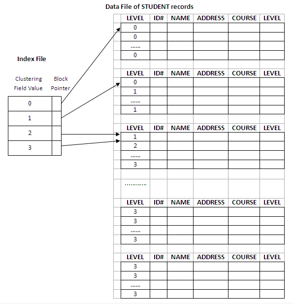
Figure 11.7
In the above figure, there are four distinct values for LEVEL: 0, 1, 2 and 3. Thus, there are four entries in the clustering index. As can be seen from the figure, many different records have the same LEVEL number and can be stored in different blocks. Both LEVEL 2 and LEVEL 3 entries point to the third block, because it stores the first record for LEVEL 2 as well as LEVEL 3 students. All other blocks following the third block must contain LEVEL 3 records, because all the records are ordered by LEVEL.
Performance improvements can be obtained by using the index to locate a record. However, the record insertion and deletion still causes similar problems to those in primary indexes, because the data records are physically ordered.
To alleviate the problem of insertion, it is common to reserve a whole block for each distinct value of the clustering field; all records with that value are placed in the block. If more than one block is needed to store the records for a particular value, additional blocks are allocated and linked together. To link blocks, the last position in a block is reserved to hold a block pointer to the next block. If there is no following block, then the block pointer will have null value.
Using this linked-blocks structure, no records with different clustering field values can be stored in the same block. It also makes insertion and deletion more efficient than without the linked structure. More blocks will be needed to store records and some spaces may be wasted. That is the price to pay for improving insertion efficiency. The figure below explains the scheme:
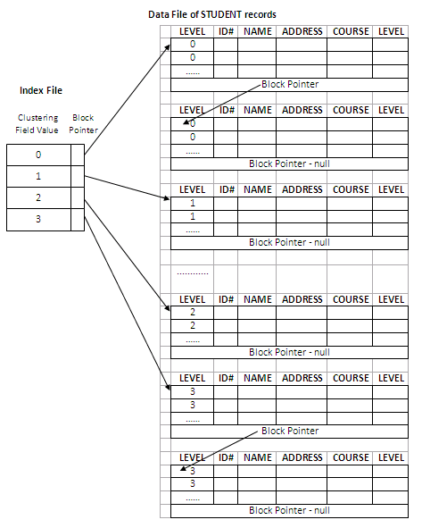
Figure 11.8
A clustering index is another type of sparse index, because it has an entry for each distinct value of the clustering field rather than for every record in the file.
A secondary index is a sorted file of records (either fixed-length or variable-length) with two fields. The first field is of the same data type as an indexing field (i.e. a non-ordering field on which the index is built). The second field is either a block pointer or a record pointer. A file may have more than one secondary index.
In this section, we consider two cases of secondary indexes:
The index access structure constructed on a key field.
The index access structure constructed on a non-key field.
Before we proceed, it must be emphasised that a key field is not necessarily an ordering field. In the case of a clustering index, the index is built on a non-key ordering field.
When the key field is not the ordering field, a secondary index can be constructed on it where the key field can also be called a secondary key (in contrast to a primary key where the key field is used to build a primary index). In such a secondary index, there is one index entry for each record in the data file, because the key field (i.e. the indexing field) has a distinct value for every record. Each entry contains the value of the secondary key for the record and a pointer either to the block in which the record is stored or to the record itself (a pointer to an individual record consists of the block address and the record’s position in that block).
A secondary index on a key field is a dense index, because it includes one entry for every record in the data file.
We again use notation <K(i), P(i)> to represent an index entry i. All index entries are ordered by value of K(i), and therefore a binary search can be performed on the index.
Because the data records are not physically ordered by values of the secondary key field, we cannot use block anchors as in primary indexes. That is why an index entry is created for each record in the data file, rather than for each block. P(i) is still a block pointer to the block containing the record with the key field value K(i). Once the appropriate block is transferred to main memory, a further search for the desired record within that block can be carried out.
A secondary index usually needs more storage space and longer search time than does a primary index, because of its larger number of entries. However, much greater improvement in search time for an arbitrary record can be obtained by using the secondary index, because we would have to do a linear search on the data file if the secondary index did not exist. For a primary index, we could still use a binary search on the main data file, even if the index did not exist. Example 2 explains the improvement in terms of the number of blocks accessed when a secondary index is used to locate a record.
Example 2
Consider the file in Example 1 with r = 40,000 records stored on a disk with block size B = 1024 bytes. File records are of fixed-length and are unspanned, with a record size R = 100 bytes. As calculated previously, this file has b = 4000 blocks. To do a linear search on the file, we would require b/2 = 4000/2 = 2000 block accesses on average to locate a record.
Now suppose that we construct a secondary index on a non-ordering key field of the file that is V = 11 bytes long. As in Example 1, a block pointer is P = 8 bytes long. Thus, the size of an index entry is Ri = (11 + 8) = 19 bytes, and the blocking factor for the index file is bfri = #(B/Ri)## = # (1024/19) ## = 53 entries per block. In a dense secondary index like this, the total number of index entries ri is equal to the number of records in the data file, which is 40000. The number of blocks needed for the index is hence bi = #(ri/bfri)## = #(40000/53)## = 755 blocks. Compare this to the 76 blocks needed by the sparse primary index in Example 1.
To perform a binary search on the index file would need #(log2bi)## = #(log2755)## = 10 block accesses. To search for the actual data record using the index, one additional block access is needed. In total, we need 10 + 1 = 11 block accesses, which is a huge improvement over the 2000 block accesses needed on average for a linear search on the data file.
Using the same principles, we can also build a secondary index on a non-key field of a file. In this case, many data records can have the same value for the indexing field. There are several options for implementing such an index.
Option 1: We can create several entries in the index file with the same K(i) value – one for each record sharing the same K(i) value. The other field P(i) may have different block addresses, depending on where those records are stored. Such an index would be a dense index.
Option 2: Alternatively, we can use variable-length records for the index entries, with a repeating field for the pointer. We maintain a list of pointers in the index entry for K(i) – one pointer to each block that contains a record whose indexing field value equals K(i). In other words, an index entry will look like this: <K(i), [P(i, 1), P(i, 2), P(i, 3), ......]>. In either option 1 or option 2, the binary search algorithm on the index must be modified appropriately.
Option 3: This is the most commonly adopted approach. In this option, we keep the index entries themselves at a fixed-length and have a single entry for each indexing field value. Additionally, an extra level of indirection is created to handle the multiple pointers. Such an index is a sparse scheme, and the pointer P(i) in index entry <K(i), P(i)> points to a block of record pointers (this is the extra level); each record pointer in that block points to one of the data file blocks containing the record with value K(i) for the indexing field. If some value K(i) occurs in too many records, so that their record pointers cannot fit in a single block, a linked list of blocks is used. The figure below explains this option.
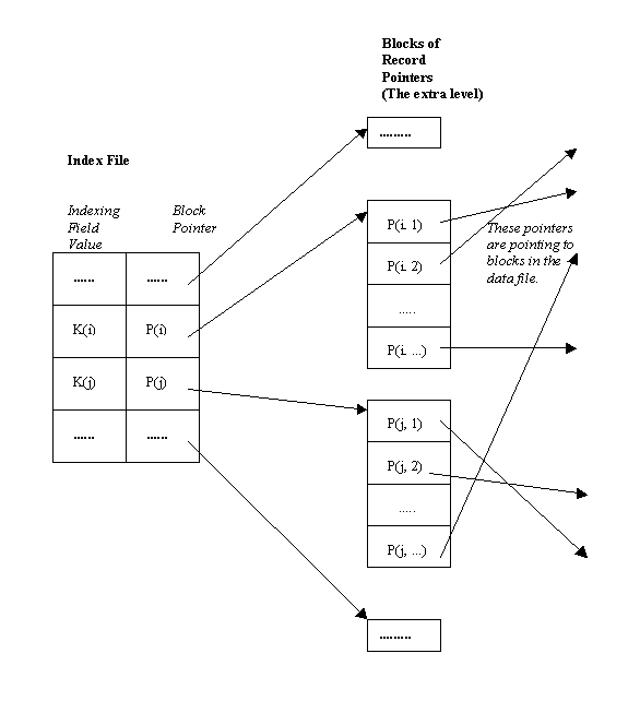
Figure 11.9
From the above figure, it can be seen that instead of using index entries like <K(i), [P(i, 1), P(i, 2), P(i, 3), ......]> and <K(j), [P(j, 1), P(j, 2), P(j, 3), ......]> as in option 2, an extra level of data structure is used to store the record pointers. Effectively, the repeating field in the index entries of option 2 is removed, which makes option 3 more appealing.
It should be noted that a secondary index provides a logical ordering on the data records by the indexing field. If we access the records in order of the entries in the secondary index, the records can be retrieved in order of the indexing field values.
The following table summarises the properties of each type of index by comparing the number of index entries and specifying which indexes are dense or sparse and which use block anchors of the data file.
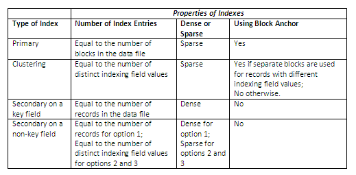
Figure 11.10
Review question 5
What are a primary index, a clustering index and a secondary index?
What is a dense index and what is a sparse index?
Why can we have at most one primary or clustering index on a file, but several secondary indexes?
Why does a secondary index need more storage space and longer search time than a primary index?
What is the major problem with primary and clustering indexes?
Why does a secondary index provide a logical ordering on the data records by the indexing field?
Exercise 5
Consider the same disk file as in Exercise 4. Answer the following questions (you need to utilise the results from Exercise 4):
Suppose the key field ID# is NOT the ordering field, and we want to build a secondary index on ID#. Is the index a sparse one or a dense one, and why?
What is the total number of index entries? How many index blocks are needed (if using block pointers to the data file)?
Determine the number of block accesses needed to search for and retrieve a record from the file using the secondary index, if the indexing field value is given.
The index structures that we have studied so far involve a sorted index file. A binary search is applied to the index to locate pointers to a block containing a record (or records) in the file with a specified indexing field value. A binary search requires #log2bi)# block accesses for an index file with bi blocks, because each step of the algorithm reduces the part of the index file that we continue to search by a factor of 2. This is why the log function to the base 2 is used.
The idea behind a multilevel index is to reduce the part of the index that we have to continue to search by bfri, the blocking factor for the index, which is almost always larger than 2. Thus, the search space can be reduced much faster. The value of bfri is also called the fan-out of the multilevel index, and we will refer to it by the notation fo. Searching a multilevel index requires #log2bi)# block accesses, which is a smaller number than for a binary search if the fan-out is bigger than 2.
A multilevel index considers the index file, which was discussed in the previous sections as a single-level ordered index and will now be referred to as the first (or base) level of the multilevel structure, as a sorted file with a distinct value for each K(i). Remember we mentioned earlier that an index file is effectively a special type of data file with two fields. Thus, we can build a primary index for an index file itself (i.e. on top of the index at the first level). This new index to the first level is called the second level of the multilevel index.
Because the second level is a primary index, we can use block anchors so that the second level has one entry for each block of the first-level index entries. The blocking factor bfri for the second level – and for all subsequent levels – is the same as that for the first-level index, because all index entries are of the same size; each has one field value and one block address. If the first level has r1 entries, and the blocking factor – which is also the fan-out – for the index is bfri = fo, then the first level needs #(r1/fo)# blocks, which is therefore the number of entries r2 needed at the second level of the index.
The above process can be repeated and a third-level index can be created on top of the second-level one. The third level, which is a primary index for the second level, has an entry for each second-level block. Thus, the number of third-level entries is r3 = #(r2/fo)#. (Important note: We require a second level only if the first level needs more than one block of disk storage, and similarly, we require a third level only if the second level needs more than one block.)
We can continue the index-building process until all the entries of index level d fit in a single block. This block at the dth level is called the top index level (the first level is at the bottom and we work our way up). Each level reduces the number of entries at the previous level by a factor of fo – the multilevel index fan-out – so we can use the formula 1 # (r1/((fo)d)) to calculate d. Hence, a multilevel index with r1 first-level entries will need d levels, where d = #(logfo(r1))#.
Important
The multilevel structure can be used on any type of index, whether it is a primary, a clustering or a secondary index, as long as the first-level index has distinct values for K(i) and fixed-length entries. The figure below depicts a multilevel index built on top of a primary index.
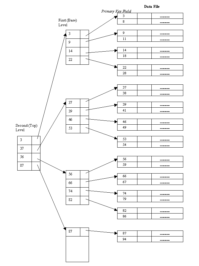
Figure 11.11
It can be seen above that the data file is a sorted file on the key field. There is a primary index built on the data file. Because it has four blocks, a second-level index is created which fits in a single block. Thus, the second level is also the top level.
Multilevel indexes are used to improve the performance in terms of the number of block accesses needed when searching for a record based on an indexing field value. The following example explains the process.
Example 3
Suppose that the dense secondary index of Example 2 is converted into a multilevel index. In Example 2, we have calculated that the index blocking factor bfri = 53 entries per block, which is also the fan-out for the multilevel index. We also knew that the number of first-level blocks b1 = 755. Hence, the number of second-level blocks will be b2 = #(b1/fo)## = #(755/53)### = 15 blocks, and the number of third-level blocks will be b3 = #(b2/fo)### = #(15/53)### = 1 block. Now at the third level, because all index entries can be stored in a single block, it is also the top level and d = 3 (remember d = #(logfo(r1))
### = #(log53(40000))### = 3, where r1 = r = 40000).
To search for a record based on a non-ordering key value using the multilevel index, we must access one block at each level plus one block from the data file. Thus, we need d + 1 = 3 + 1 = 4 block accesses. Compare this to Example 2, where 11 block accesses were needed when a single-level index and binary search were used.
Note
It should be noted that we could also have a multilevel primary index which could be sparse. In this case, we must access the data block from the file before we can determine whether the record being searched for is in the file. For a dense index, this can be determined by accessing the first-level index without having to access the data block, since there is an index entry for every record in the file.
As seen earlier, a multilevel index improves the performance of searching for a record based on a specified indexing field value. However, the problems with insertions and deletions are still there, because all index levels are physically ordered files. To retain the benefits of using multilevel indexing while reducing index insertion and deletion problems, database developers often adopt a multilevel structure that leaves some space in each of its blocks for inserting new entries. This is called a dynamic multilevel index and is often implemented by using data structures called B-trees and B+ trees, which are to be studied in the following sections.
Review question 6
How does the multilevel indexing structure improve the efficiency of searching an index file?
What are the data file organisations required by multilevel indexing?
Exercise 6
Consider a disk with block size B = 512 bytes. A block pointer is P = 8 bytes long, and a record pointer is Pr = 9 bytes long. A file has r = 50,000 STUDENT records of fixed-size R = 147 bytes. The key field ID# has a length V = 12 bytes. (This is the same disk file as in Exercise 4 and 5. Previous results should be utilised.) Answer the following questions:
Suppose the key field ID# is the ordering field, and a primary index has been constructed (as in Exercise 4). Now if we want to make it into a multilevel index, what is the number of levels needed and what is the total number of blocks required by the multilevel index?
Suppose the key field ID# is NOT the ordering field, and a secondary index has been built (as in Exercise 5). Now if we want to make it into a multilevel index, what is the number of levels needed and what is the total number of blocks required by the multilevel index?
B-trees and B+ trees are special types of the well-known tree data structure. A tree is formed of nodes. Each node in the tree, except for a special node called the root, has one parent node and any number (including zero) of child nodes. The root node has no parent. A node that does not have any child nodes is called a leaf node; a non-leaf node is called an internal node.
The level of a node is always one more than the level of its parent, with the level of the root node being zero. A sub-tree of a node consists of that node and all its descendant nodes (i.e. its child nodes, the child nodes of its child nodes, and so on). The figure below gives a graphical description of a tree structure:
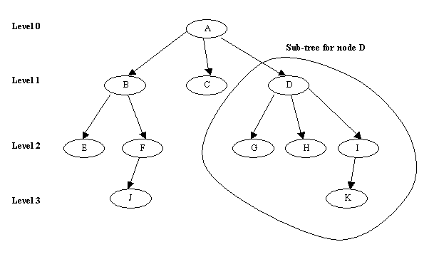
Figure 11.12
Usually we display a tree with the root node at the top. One way to implement a tree is to have as many pointers in each node as there are child nodes of that node. In some cases, a parent pointer is also stored in each node. In addition to pointers, a node often contains some kind of stored information. When a multilevel index is implemented as a tree structure, this information includes the values of the data file’s indexing field that are used to guide the search for a particular record.
A search tree is a special type of tree that is used to guide the search for a record, given the value of one of its fields. The multilevel indexes studied so far can be considered as a variation of a search tree. Each block of entries in the multilevel index is a node. Such a node can have as many as fo pointers and fo key values, where fo is the index fan-out.
The index field values in each node guide us to the next node (i.e. a block at the next level) until we reach the data file block that contains the required record(s). By following a pointer, we restrict our search at each level to a sub-tree of the search tree and can ignore all other nodes that are not in this sub-tree.
A search tree of order p is a tree such that each node contains at most p – 1 search values and p pointers in the order <P1, K1, P2, K2, ......, Pq-1, Kq-1, Pq>, where p and q are integers and q # p.
Each Pi is a pointer to a child node (or a null pointer in the case of a leaf node), and each Ki is a search value from some ordered set of values. All search values are assumed unique. The figure below depicts in general a node of a search tree:
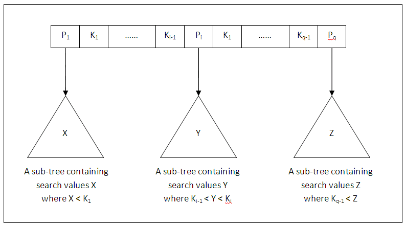
Figure 11.13
Two constraints must hold at all times on the search tree:
Within each node (internal or leaf), K1 < K2 < ...... < Kq-1.
For all values X in the sub-tree pointed at by Pi, we must have Ki-1 < X < Ki for 1 < i < q; X < Ki for i = 1; and Ki-1 < X for i = q.
Whenever we search for a value X, we follow the appropriate pointer Pi according to the formulae in the second condition above.
A search tree can be used as a mechanism to search for records stored in a disk file. The values in the tree can be the values of one of the fields of the file, called the search field (same as the indexing field if a multilevel index guides the search). Each value in the tree is associated with a pointer to the record in the data file with that value. Alternatively, the pointer could point to the disk block containing that record.
The search tree itself can be stored on disk by assigning each tree node to a disk block. When a new record is inserted, we must update the search tree by including in the tree the search field value of the new record and a pointer to the new record (or the block containing the record).
Algorithms are essential for inserting and deleting search values into and from the search tree while maintaining the two constraints. In general, these algorithms do not guarantee that a search tree is balanced (balanced means that all of the leaf nodes are at the same level). Keeping a search tree balanced is important because it guarantees that no nodes will be at very high levels and hence require many block accesses during a tree search. Another problem with unbalanced search trees is that record deletion may leave some nodes in the tree nearly empty, thus wasting storage space and increasing the number of levels.
Please note that you will not be expected to know the details of given algorithms in this chapter, as the assessment will focus on the advantages and disadvantages of indexing for performance tuning. The algorithms are only provided for the interested reader.
Review question 7
Describe the tree data structure.
What is meant by tree level and what is a sub-tree?
A B-tree is a search tree with some additional constraints on it. The additional constraints ensure that the tree is always balanced and that the space wasted by deletion, if any, never becomes excessive.
For a B-tree, however, the algorithms for insertion and deletion become more complex in order to maintain these constraints. Nonetheless, most insertions and deletions are simple processes; they become complicated when we want to insert a value into a node that is already full or delete a value from a node which is just half full. The reason is that not only must a B-tree be balanced, but also, a node in the B-tree (except the root) cannot have too many (a maximum limit) or too few (half the maximum) search values.
A B-tree of order p is a tree with the following constraints:
Each internal node is of the form <P1, <K1, Pr1>, P2, <K2, Pr2>, ......, Pq-1, <Kq-1, Prq-1>, Pq> where q <= p. Each Pi is a tree pointer – a pointer to another node in the B-tree. Each Pri is a data pointer – a pointer to the block containing the record whose search field value is equal to Ki.
Within each node, K1 < K2 < ...... < Kq-1.
For all search key field values X in the sub-tree pointed at by Pi, we have Ki-1 < X < Ki for 1 < i < q; X < Ki for i = 1; Ki-1 < X for i = q.
Each node has at most p tree pointers and p –1 search key values (p is the order of the tree and is the maximum limit).
Each node, except the root and leaf nodes, has at least #(p/2)# tree pointers and #(p/2)# - 1 search key values (i.e. must not be less than half full). The root node has at least two tree pointers (one search key value) unless it is the only node in the tree.
A node with q tree pointers, q # p, has q – 1 search key field values (and hence has q – 1 data pointers).
All leaf nodes are at the same level. They have the same structure as internal nodes except that all of their tree pointers Pi are null.
The figure below illustrates the general structure of a node in a B-tree of order p:
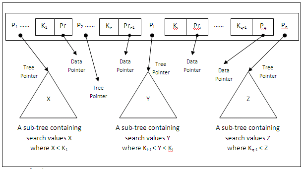
Figure 11.14
The figure below shows a B-tree of order 3:
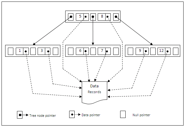
Figure 11.15
Notice that all search values K in the B-tree are unique because we assumed that the tree is used as an access structure on a key field. If we use B-tree on a non-key field, we must change the definition of the data pointers Pri to point to a block (or a linked list of blocks) that contain pointers to the file records themselves. This extra level of indirection is similar to Option 3 discussed before for secondary indexes.
A B-tree starts with a single root node at level 0. Once the root node is full with p – 1 search key values, an insertion will cause an overflow and the node has to be split to create two additional nodes at level 1 (i.e. a new level is created). Only the middle key value is kept in the root node, and the rest of the key values are redistributed evenly between the two new nodes.
When a non-root node is full and a new entry is inserted into it, that node is split to become two new nodes at the same level, and the middle key value is moved to the parent node along with two tree pointers to the split nodes. If such a move causes an overflow in the parent node, the parent node is also split (in the same way). Such splitting can propagate all the way to the root node, creating a new level every time the root is split. We will study the algorithms in more details when we discuss B+ trees later on.
Deletion may cause an underflow problem, where a node becomes less than half full. When this happens, the underflow node may obtain some extra values from its adjacent node by redistribution, or may be merged with one of its adjacent nodes if there are not enough values to redistribute. This can also propagate all the way to the root. Hence, deletion can reduce the number of tree levels.
It has been shown by analysis and simulation that, after numerous random insertions and deletions on a B-tree, the nodes are approximately 69% full when the number of values in the tree stabilises. This is also true of B+ trees. If this happens, node splitting and merging will occur rarely, so insertion and deletion become quite efficient. If the number of values increases, the tree will also grow without any serious problem.
The following two examples show us how to calculate the order p of a B-tree stored on disk (Example 4), and how to calculate the number of blocks and levels for the B-tree (Example 5).
Example 4
Suppose the search key field is V = 9 bytes long, the disk block size is B = 512 bytes, a data pointer is Pr = 7 bytes, and a block pointer is P = 6 bytes. Each B-tree node can have at most p tree pointers, p – 1 search key field values, and p – 1 data pointers (corresponding to the key field values). These must fit into a single disk block if each B-tree node is to correspond to a disk block. Thus, we must have
(p * P) + ((p – 1) * (Pr + V)) # B
That is (p * 6) + ((p – 1) * (7 + 9)) # 512
We have (22 * p) # 528
We can select p to be the largest value that satisfies the above inequality, which gives p = 24.
In practice, the value of p will normally be smaller than 24 (e.g., p = 23). The reason is that, in general, a B-tree node may contain additional information needed by the algorithms that manipulate the tree, such as the number of entries q in the node and possibly a pointer to the parent node. Thus, we should reduce the block size by the amount of space needed for all such information before we determine the value of p.
Example 5
Suppose that the search field of Example 4 is a non-ordering key field, and we construct a B-tree on this field. Assume that each node of the tree is 69% full. On average, therefore, each node will have p * 0.69 = 23 * 0.69 @ 16 pointers, and hence 15 search key field values. The average fan-out fo = 16.
We can now start from the root and see how many values and pointers may exist, on average, at each subsequent level (see the table below):
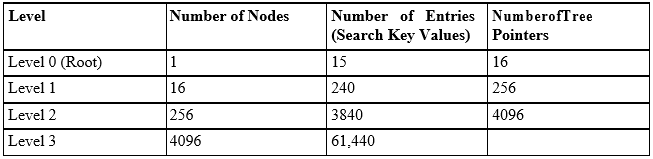
Figure 11.16
At each level, we calculate the number of entries by multiplying the total number of pointers at the previous level by 15 – the average number of entries in each node. Hence, for the given block size, pointer size, and search key field size (as in Example 5), a two level B-tree can hold up to 3840 + 240 + 15 = 4095 entries; a three-level B-tree can hold up to 61440 + 3840 + 240 + 15 = 65,535 entries on average.
Most implementations of a dynamic multilevel index use a variation of the B-tree data structure, called a B+ tree. In a B-tree, every value of the search field appears once at some level in the tree, along with a corresponding data pointer. In a B+ tree, data pointers are stored only at the leaf nodes of the tree; hence, the structure of leaf nodes differs from that of internal nodes.
The leaf nodes have an entry for every value of the search field, along with a corresponding data pointer to the block containing the record with that value if the search field is a key field. For a non-key search field, the pointer points to a block containing pointers to the data file records, creating an extra level of indirection (as we have seen before).
The leaf nodes of a B+ tree are usually linked together to provide ordered access on the search field to the records. These leaf nodes are similar to the first level of a multilevel index. Internal nodes correspond to the other levels of the multilevel index. Some search field values from the leaf nodes are duplicated in the internal nodes to guide the search.
The structure of the internal nodes of a B+-tree of order p is defined as follows:
Each internal node is of the form: <P1, K1, P2, K2, ......, Pq-1, Kq-1, Pq> where q <= p and each Pi is a tree pointer.
Within each internal node, K1 < K2 < ...... < Kq-1.
For all search field values X in the sub-tree pointed at by Pi, we have
Ki-1 < X <= Ki for 1 < i < q;
X <= Ki for i = 1;
Ki-1 < X for i = q.
Each internal node has at most p tree pointers and p –1 search key values.
Each internal node, except the root, has at least #(p/2)# tree pointers and #p/2)# - 1 search key values (i.e. must not be less than half full). The root node has at least two tree pointers (one search key value) if it is an internal node.
An internal node with q tree pointers, q # p, has q – 1 search key field values.
The structure of the leaf nodes of a B+ tree of order p is defined as follows:
Each leaf node is of the form <<K1, Pr1>, <K2, Pr2>, ......, <Kq-1, Prq-1>, Pnext> where q # p. Each Pri is a data pointer, and Pnext points to the next leaf node of the B+ tree.
Within each internal node, K1 < K2 < ...... < Kq-1.
Each Pri is a data pointer pointing to the record whose search field value is Ki, or to a file block containing the record (or to a block of record pointers that point to records whose search field value is Ki, if the search field is not a key).
Each leaf node has at least #(p/2)# values (entries).
All leaf nodes are at the same level.
The following figure depicts the general structure of an internal node of a B+ tree of order p:
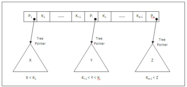
Figure 11.17
And the following figure depicts the general structure of a leaf node of a B+ tree of order p:
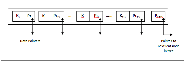
Figure 11.18
Because entries in the internal nodes just contain search values and tree pointers without any data pointers, more entries can be accommodated into an internal node of a B+ tree than for a similar B-tree. Thus, for the same block (node) size, the order p can be larger for the B+ tree than for a B-tree (see Example 6). This can lead to fewer B+ tree levels, and therefore improve search time.
Because structures of internal nodes and leaf nodes are different, their orders can be different. Generally, the order p is for the internal nodes, and leaf nodes can have a different order denoted as pleaf, which is defined as being the maximum number of data pointers in a leaf node.
Example 6
To calculate the order p of a B+tree, suppose that the search key field is V = 9 bytes long, the block size is B = 512 bytes, a record (data) pointer is Pr = 7 bytes, and a block pointer is P = 6 bytes, all as in Example 4. An internal node of such a B+-tree can have up to p tree pointers and p – 1 search field values: these must fit into a single block. Hence, we have
(p * P) + ((p – 1) * V) # B
That is (p * 6) + ((p – 1) * 9) # 512
We have (15 * p) # 521
We can select p to be the largest value that satisfies the above inequality, which gives p = 34. This is larger than the value of 23 for the B-tree in Example 5, resulting in a larger fan-out and more entries in each of the internal nodes.
The leaf nodes of the B+tree will have the same number of values and pointers, except that the pointers are data pointers and one Pnext pointer (i.e., a block pointer to another leaf node). Hence, the order pleaf for the leaf nodes can be calculated similarly:
(pleaf * (Pr + V)) + P # B
That is (pleaf * (7 + 9)) + 6 # 512
We have (16 * pleaf) # 506
It follows that each leaf node can hold up to pleaf = 31 (key value, data pointer) pairs.
As with B-tree, in practice, the value of p and pleaf will normally be smaller than the above values. The reason is that, in general, we may need additional information in each node to implement the insertion and deletion algorithms. This kind of information can include the type of nodes (i.e., internal or leaf), the number of current entries q in the node, and pointers to the parent and sibling nodes (e.g., Pprevious). Thus, we should reduce the block size by the amount of space needed for all such information before we determine the values of p and pleaf.
The next example explains how we can calculate the number of entries in a B+tree.
Example 7
Suppose that we want to build a B+tree on the field of Example 6. To calculate the approximate number of entries of the B+-tree, we assume that each node is 69% full. On average, each internal node will have 0.69 * p = 0.69 * 34 = 23 pointers and hence 22 values. Each leaf node, on average, will hold 0.69 * pleaf = 0.69 * 31 = 21 data record pointers. Such a B+-tree will have the following average number of entries at each level:
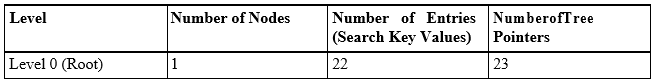
Figure 11.19
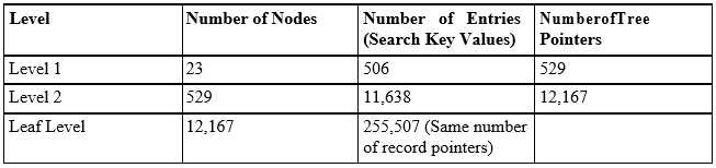
Figure 11.20
For the block size, pointer size, and search field size provided above, a three-level B+tree holds up to 255,507 record pointers, on average. Compare this to the 65,535 entries for the corresponding B-tree in Example 6. It is apparent that a B+tree is more efficient.
To search for a record based on a specified search field value K:
We always start from the root of the B+ tree. Compare K with the values stored in the root until we find the first Ki where K <= Ki. Then follow the tree pointer Pi to the next level. If no such Ki is found, then follow the rightmost pointer Pq to the next level. (We assume that the root is not the only node in the tree. Otherwise follow the search procedure for a leaf node.)
If the node at the next level is still an internal node, we repeat the above procedure, until we reach the leaf level.
Within a leaf node, we search for a stored value Ki that equals K. If found, we follow its data pointer Pri to retrieve the data block. Otherwise, the desired record is not in the file.
The following is an example of a B+ tree with p = 3 and pleaf = 2:
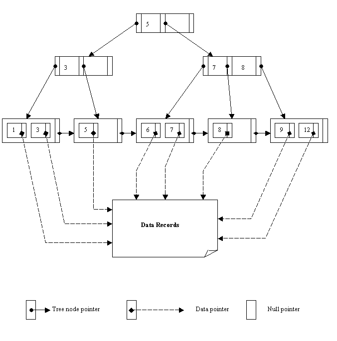
Figure 11.21
Refer to the tree above. Suppose we want to retrieve the record with value 6 in the search field. Having searched the root, we could not find a value Ki such that 6 # Ki, because there is only one value 5 in the node. Thus, we follow the rightmost pointer to the internal node at the next level. This node has two values 7 and 8, but 7 is the first value that is bigger than 6. Hence, we follow the pointer left to the value 7 to the leaf level. By searching the values in the leaf node, we find the value 6. Then we will use the related data pointer to go to the data file and retrieve the record.
Note that every distinct search value must exist at the leaf level, because all data pointers are at the leaf level. However, only some of the search values exist in internal nodes, to guide the search to reach the appropriate leaf node. Also note that every value appearing in an internal node also appears as the rightmost value in the sub-tree pointed at by the tree pointer to the left of the value. In the above, for example, the value 5 in the root node (an internal node as well) is also stored in the sub-tree pointed at by the left pointer. The value 5 is in the leaf node of the sub-tree and is the rightmost value. The same is true for other values in the internal nodes, such as 3, 7 and 8.
Insertion and deletion of entries in a B+ tree can cause the same overflow and underflow problems as for a B-tree, because of the restrictions (constraints) imposed by the B+ tree definition. These problems are dealt with in a similar way as in a B-tree, i.e. by splitting or merging nodes concerned.
When a leaf node overflows because of insertion of a new entry, it must be split. The first m = #((pleaf + 1)/2)# entries in the original node are kept there, and the rest are moved to a new leaf node (just created).
The original pnext pointer is changed and points to the new leaf node, and the same pointer new_pnext in the new node will have the original value of pnext.
The mth search value is duplicated in the parent node (an internal node), and an extra pointer to the new node is created in the parent.
If the above move of value causes overflow in the parent node because the parent node is already full, then it must also split.
A new internal node will now hold the entries from Pn+1 to the end of the entries in the overflowed node.
This splitting can propagate all the way up to create a new root node and hence a new level for the B+ tree.
When an entry is deleted, it is always removed from the leaf level. If it happens to occur in an internal node (because it is the rightmost value of a sub-tree), then it must also be removed from there. In this case, the value to its left in the leaf node will replace it in the internal node, because that node is now the rightmost entry in the sub-tree.
If deletion causes underflow, we will try to find an adjacent leaf node and redistribute the entries among the two nodes so that both can become at least half full.
If we cannot find such an adjacent node with enough entries, then we will merge them. In this case, the number of leaf nodes is reduced.
If a merge between two nodes is not possible because of insufficient number of entries, we may merge three leaf nodes into two.
In merge cases, underflow may propagate to internal nodes because one fewer tree pointer and search value are needed. This can propagate to the root and reduce the tree levels.
The algorithms for maintaining a B+ tree structure are necessarily complex, and therefore some operational details are omitted in this chapter. However, such algorithms are well established and tested, and their efficiency proved. Interested students are advised to read the relevant chapters in the recommended textbooks for details.
Recall that the definitions of B-tree and B+ tree require each node to be at least half full. Such a requirement can be changed to require each node to be at least two-thirds full. In this case, the B-tree is called a B*tree. This can improve the retrieval performance a little further without incurring too many overheads on maintaining the tree.
Exercise 7
Consider the disk with block size B = 512 bytes. A block pointer is P = 8 bytes long, and a record pointer is Pr = 9 bytes long. A file has r = 50,000 STUDENT records of fixed-size R = 147 bytes. The key field is ID# whose length is V = 12 bytes. (This is the same disk file as in previous exercises. Some of the early results should be utilised.) Suppose that the file is NOT sorted by the key field ID# and we want to construct a B-tree access structure (index) on ID#. Answer the following questions:
What is an appropriate order p of this B-tree?
How many levels are there in the B-tree if nodes are approximately 69% full?
What is the total number of blocks needed by the B-tree if they are approximately 69% full?
How many block accesses are required to search for and retrieve a record from the data file, given an ID#, using the B-tree?
Exercise 8
For the same disk file as in Exercise 7, suppose that the file is NOT sorted by the key field ID# and we want to construct a B+tree access structure (index) on ID#. Answer the following questions:
What are the appropriate order p (for internal nodes) and pleaf (for leaf nodes) of this B+-tree?
How many leaf-level blocks are needed if blocks are approximately 69% full?
How many levels are there if internal nodes are also 69% full?
How many block accesses are required to search for and retrieve a record from the data file, given an ID#, using the B+tree?
B-trees/B+ trees/B* trees are data structures which can be used to implement dynamic multilevel indexes very effectively. When we were discussing multilevel indexes, we emphasised that the multilevel structure can be constructed for any type of index, whether it is a primary, a clustering or a secondary index, as long as the first-level index has distinct values for K(i) and fixed-length.
As a logical consequence of the above, the multilevel index structure does not require the underlying data file to have any specific file organisation, i.e. it can be a heap file, a sorted file or some other organisations.
Also recall that a heap file organisation is very efficient with regard to insertion and deletion, but less efficient for retrieval. Such inefficiency for retrieval can be overcome by building a multilevel index structure on top of it. A heap file with a multilevel index is, therefore, a very effective combination that takes full advantage of different techniques while overcoming their respective shortcomings. The figure below illustrates the combination:
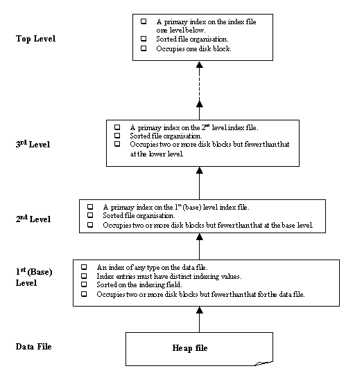
Figure 11.22
Review question 8
Describe the general structure of a B-tree node. What is the order p of a B-tree?
Describe the structure of both internal and leaf nodes of a B+ tree. What is the order p of a B+ tree?
Why is a B+ tree usually preferred as an access structure to a data file rather than a B-tree?
In a B+ tree structure, how many block accesses do we need before a record is located? (Assuming the record is indeed in the data file and its indexing field value is specified.)
What major problems may be caused by update operations on a B-tree/B+ tree structure and why?