Figure 18.1
Table of contents
Almost all database applications are concerned with the modelling and storage of data that varies with time. It is not surprising therefore, that a great deal of research and development, both in industry and in universities, has gone into developing database systems that support the time-related or temporal aspects of data processing. In this chapter we shall examine the major issues in the provision of support for temporal data. We shall explore some of the most important research that has been done in the area, and identify the influence of this research on query languages.
At the end of this chapter you should be able to:
Define and use important temporal concepts, such as time point, time interval, and time-interval operators such as before, after and overlaps.
Explain the issues involved in modelling a number of time-varying features of data, such as transaction time, valid time and time granularity.
Understand the temporal data model at the conceptual level.
Describe some of the extensions to conventional query languages that have been proposed to support temporal query processing.
Detailed concepts of temporal databases can be found in the book titled “Time and Relational Theory (Temporal Databases in the Relational Model and SQL), 2nd Edition by C.J. Date, Hugh Darwen and Nikos Lorentzos”
A temporal database is generally understood as a database capable of supporting storage and reasoning of time-based data. For example, medical applications may be able to benefit from temporal database support — a record of a patient's medical history has little value unless the test results, e.g. the temperatures, are associated to the times at which they are valid, since we may wish to do reasoning about the periods in time in which the patient’s temperature changed.
Temporal databases store temporal data, i.e. data that is time dependent (timevarying). Typical temporal database scenarios and applications include time-dependent/time-varying economic data, such as:
Share prices
Exchange rates
Interest rates
Company profits
The desire to model such data means that we need to store not only the respective value but also an associated date or a time period for which the value is valid. Typical queries expressed informally might include:
Give me last month's history of the Dollar-Pound Sterling exchange rate.
Give me the share prices of the NYSE on October 17, 1996.
Many companies offer products whose prices vary over time. Daytime telephone calls, for example, are usually more expensive than evening or weekend calls. Travel agents, airlines or ferry companies distinguish between high and low seasons. Sports centres offer squash or tennis courts at cheaper rate during the day. Hence, prices are time dependent in these examples. They are typically summarised in tables with prices associated with a time period.
As well as the user of a database recording when certain data values are valid, we may wish to store (for backup, or analysis reasons) historical records of changes made to the database. So each time a change to a database is made the system may automatically store a transaction timestamp. Therefore a temporal database may be storing two different pieces of time data for a tuple — the user-defined period of time for which the data is valid (e.g. October to April [winter season] rental of tennis courts are 1 US dollar per hour), and the system-generated transaction timestamp for when the tuple (or part of a tuple) was changed (e.g. 14:55 on 03/01/1999). A temporal database ability to store these different kinds of data makes possible many different kinds of temporal-based queries, as long as its query language and data model are sophisticated enough to formally model and allow reasoning about temporal data. It is the possible gains from such temporal querying facilities that has provided the motivation for research and development into extending the Relational database model for temporal data (and suggesting alternatives to the Relational model…).
Our everyday life is very often influenced by timetables for buses, trains, flights, university lectures, laboratory access and even cinema, theatre or TV programmes. As one consequence, many people plan their daily activities by using diaries, which themselves are a kind of timetable. Timetables or diaries can be regarded as temporal relations in terms of a Relational temporal data model. Medical diagnosis often draws conclusions from a patient's history, i.e. from the evolution of his/her illness. The latter is described by a series of values, such as the body temperature, cholesterol concentration in the blood, blood pressure, etc. As in the first example, each of these values is only valid during a certain period of time (e.g. a certain day). Typically a doctor would retrieve a patient's values' history, analyse trends and base diagnosis on such observations. Similar examples can be found in many areas that rely on the observation of evolutionary processes, such as environmental studies, economics and many natural sciences.
From a philosophical point of view we might argue either that time passes continuously, flowing as if a stream or river of water, or we can think of time passing in discrete units of time, each with equal duration, as we think of time when listening to the ticking of a clock. For the purposes of recording and reasoning about time, many people prefer to work with a conceptual model of time as being discrete and passing in small, measurable units; however, there are some occasions and applications where a continuous model of time is most appropriate.
When we think about time as passing in discrete units, depending on the purpose or application, different-sized units may be appropriate. So the age of volcanoes may be measured in years, or decades, or hundreds of years. The age of motor cars may be measured in years, or perhaps months for ‘young’ cars. The age of babies may be measured in years, or months, or weeks, or days. The age of bacteria in seconds or milliseconds. The size of the units of time used to refer to a particular scenario is referred to as the granularity of the temporal units — small temporal grains refer to short units of time (days, hours, seconds, milliseconds, etc), and large temporal grains refer to longer units of time (months, years, decades, etc).
For a particular situation we may wish to define the smallest unit of time which can be recorded or reasoned about. One way to refer to the chosen, indivisible unit of time is as 'time quanta'. Sometimes the term ‘chronon’ or ‘time granule’ is used to refer to the indivisible units of time quanta for a situation or system. In this chapter we shall use the term time quanta.
When attempting to represent and reason about time, four important concepts are:
Points: Formally a point in time has no duration; it simply refers to a particular position in the timeline under discussion. We can talk of the point in time at which some event begins or ends.
Duration: A duration refers to a number of time quanta; for example, a week, two months, three years and 10 seconds are all durations. A duration refers to a particular magnitude (size) of a part of a timeline, but not the direction (so whether we talk of a week ago or a week beginning in three days' time, we are still referring to a length of time of a week).
Interval: An interval has a start time point and an end time point. Using more formal notation, we can refer to an interval I(s, e) with start point ‘s’ and end point ‘e’, and for which all points referring to time from s to e (inclusive) make up the interval. Note that there is an assumption (constraint) that the timepoint ‘s’ does not occur after the timepoint ‘e’ (an interval of zero time quanta would have a start point and end point that were equal).
Timeline: Conceptually we can often imagine time as moving along a line in one direction. When graphically representing time, it is usual to draw a line (often with an arrow to show time direction), where events shown towards the end of the timeline have occurred later than those shown towards the beginning of the line. Often a graphical timeline is draw like an axis on a graph (by convention, the X-axis represents time) and the granularity of the time units is marked (and perhaps labelled) along the X-axis.
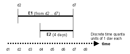
You may find the following diagram useful in illustrating these four concepts:
Figure 18.1
Looking at the figure, there are two events, E1 and E2. We see that event E1 starts at the time point ‘d2’ and ends at time point ‘d7', therefore event E1 is an example of an interval. All that is written for event E2 is that it lasts four days, so event E2 is a duration (although we might attempt to infer from the X-axis that E2 appears to start at d4 and end at d7, but perhaps E2 is four days measured back from d7). The X-axis is a labelled arrow ‘time’, and represents a timeline. There are units labelled on the X-axis from ‘d1’ to ‘d8’, and a note indicates that these units are time quanta representing one day each.
Since the time quanta are a day each for this model, we are not able to model any time units of less that one day (so even if it looked like an event started halfway between two units on the diagram, we could not meaningfully talk of day 1 plus 12 hours or whatever). This does raise an issue when attempting to convert from a model of one time granularity to anothe. For example, if all data from the model above were to be added to a database where the time quanta was in terms of hours, what hour of the day would ‘d3’ represent? Would it be midnight when the day started, or midday, or 09:00 in the morning (the start of a working day)? Such questions must be answered by any data analyst if converting between different temporal models, which is one reason why it is so important to choose an appropriate granularity of time quanta. It might seem reasonable, just in case, to choose a very small time quanta, such as seconds or milliseconds,but there may be significant memory implications for such a choice (e.g. if the database system had to use twice as much memory to record millisecond timestamps for each attribute of each tuple, rather than just recording the day timestamp).
Much of the recent work in the fields of time-based computing (both for databases and other areas such as artificial intelligence) is based on the work of J. F. Allen. A publication by Allen that is frequently cited in literature about time-based reasoning is:
Maintaining Knowledge about Temporal Intervals, J. F. Allen, CACM (Communications of the Association for Computing Machinery) Volume 16 number 11, November 1983.
Allen’s contribution to those wishing to represent and reason about time-based information consisted of the formalisation of possible relationships between pairs of intervals. Although the following, informal overview may seem obvious from an intuitive perspective, Allen presented these concepts in a rigorous, formal way which has been the basis for much temporal reasoning and computer system design since.
Consider two events, E1 and E2. Each event has a starting point in time and an ending point in time — therefore each event takes place as an interval in time. The following are the possible relationships between two intervals (events):
E1 starts and ends before E2 begins.
E1 ends at the same point in time that E2 begins — the two events are temporally contiguous. We can say that the end of E1 meets the beginning of E2.
E1 starts before E2 starts, but the end of E1 overlaps with the beginning of E2. E2 ends after E1 has ended.
E1 takes place entirely during the period that E2 exists, i.e. E1 starts after E2 and E1 finishes before E2.
E1 occurs after E2 has ended.
Both E1 and E2 may start at the same time (likewise, both E1 and E2 might finish at the same time).
Each of these relationships can be formally defined as an operation between intervallic events, and these operators are often referred to as 'Allen’s operators'. Each of the above is perhaps more easily understood in graphical representations.
• E1 BEORE E2 — E1 occurs before E2
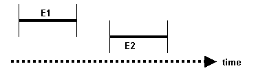
Figure 18.2
• E1 MEETS E2 — The end of E1 meets the beginning of E2
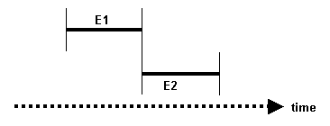
Figure 18.3
• E1 OVERLAPS E2 — E1 overlaps with E2
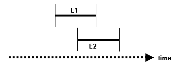
Figure 18.4
• E1 DURING E2 — E1 takes place during E2 (E1 and E1 may start and finish at the same time)
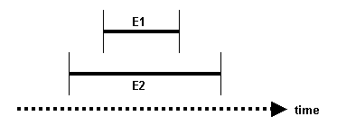
Figure 18.5
• E1 AFTER E2 — E1 occurs after E2 has ended
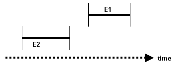
Figure 18.6
• E1 STARTS E2 — E1 starts at the same time that E2 starts (and E1 does not end after E2)
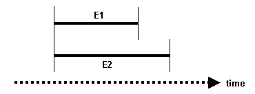
Figure 18.7
• E1 FINISHES E2 — E1 finishes at the same time that E2 ends (and E1 does not start before E2)
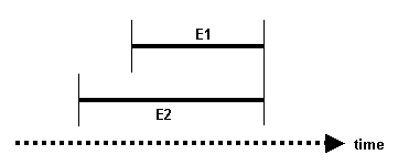
Figure 18.8
For certain formal reasoning and temporal relational operators, the concept of a unary interval is important. A unary interval has a duration of one time unit (one time quantum). For example:
Interval_A( t4, t4 )
The interval Interval_A has a start time of ‘t4’ and an end time of ‘t4’. Therefore it starts at the beginning of the time quantum t4, and ends at the end of the time quantum t4, and so has a duration of 1 time quantum. Other examples of unary intervals include:
Interval_B( t1, t1 ) Interval_C( t9, t9 ) and so on.
Any interval with start time ‘s’ and end time ‘e’ can be ‘unfolded’ into a sequence of unary intervals. For example, some Interval_D( t3, t7 ), which starts at t3 and ends at t7, can be thought of as being the same as the set of unary intervals:
( t3, t3 ) ( t4, t4 ) ( t5, t5 ) ( t6, t6 ) ( t7, t7 )
We shall return to the use of the unary interval concept when relational temporal operators are investigated.
A reference to a duration or interval can be absolute or relative to some time point or other interval. The position on the time axis of a period or of an instant can be given as an absolute position, such as the calendric time (e.g. "Blood pressure taken on 3November 1996"). This is a common approach adopted by data models underlying temporal medical databases.
However, it also is common in medicine to reason with relative time references: "Heartbeat measurement taken after a long walk", “the day after tomorrow”, etc. The relationship between times can be qualitative (before, after, etc) as well as quantitative (three days before, 397 years after, etc.). Examples include:
Mary's salary was raised yesterday.
It happened sometime last week.
It happened within three days of Easter.
The French revolution occurred 397 years after the discovery of America.
In general, the behaviour of temporal entities can be classified into one of four basic categories, namely:
Discrete
Continuous
Stepwise constant
Period based
These can be depicted graphically as shown in the figures below. We shall consider each category of temporal data individually.
Continuous behaviour is observed where an attribute value is recorded constantly over time such that its value may be constantly changing. Continuous behaviour can often be found in monitoring systems recording continuous characteristics - for example, a speedometer of a motorcar.
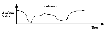
Figure 18.9
Discrete data attributes are recorded at specific points in time but have no definition at any other points in time. Discrete data is associated with individual events such as "A complete check-up was on a particular date".
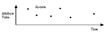
Figure 18.10
Stepwise constant data consists of values that change at a point in time, then remain constant until being changed again - for example, blood pressure measurement.
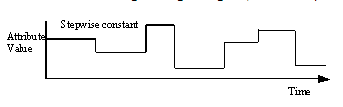
Figure 18.11
Period-based data models the behaviour of events that occur over some period of time but, at the end of this period, become undefined. An example of period-based data would be patient drug usage records, where a patient takes a drug for a prescribed period of time and then stops taking it.
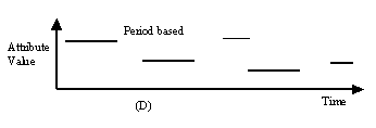
Figure 18.12
Exercises
Exercise 1 - Temporal terms and concepts
State whether each of the following is a point, duration or interval:
10 seconds
14.45 on 3/Feb/2007
Three days
From 1/3/99 to 5/1/99
Exercise 2 - Granularity
Which is the smaller level of temporal granularity: seconds or days?
Exercise 3 - Time quanta
What are time quanta? Are seconds or days examples of time quanta?
Exercise 4 - Interval operators
Consider the following scenario:
the time E1 starts is t2, i.e. s1=t2
the time E1 ends is t7, i.e. e1=t7
the time E2 starts is t5=t4, i.e. s2=t7
the time E2 ends is t7, i.e. e2=t7
In terms of Allen’s operators, what can we say about the relationship(s) between E1 and E2?
Draw a diagram showing the two events on the timeline t1, t2, … t8, to illustrate the relationship between the intervals.
Exercise 5 - Relative and absolute time
Which of the following are absolute and which are relative times?
7th May 1991
The day after tomorrow
14:13 on Monday 14th April 2010
A week after last Tuesday
10 minutes after we finish work
Exercise 6 - Category of temporal data behaviour
What kind of temporal data behaviour does the following graph represent?
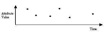
Figure 18.13
A database might be informally defined as a collection of related data. This data corresponds to some piece of the Universe of Discourse (UoD) — i.e. the data we record represents a model of those parts of the real world (or an imagined world) which we are interested in, and wish to reason about. An example of a Universe of Discourse might be the patients, doctors, operating theatres, booked operations and available drugs in a hospital. Another UoD might be a basketball competition made up of each team, player, set of fixtures and results of games played to date.
The figure below illustrates that at a particular point in time, the Universe of Discourse is in a particular state, and we create a database at this point in time recording details of the state of the UoD:
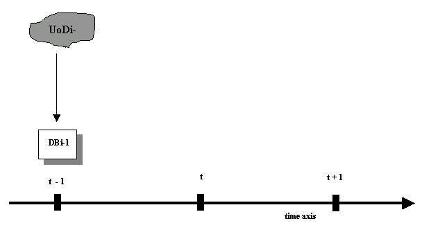
Figure 18.14
As time passes, the UoD is subject to events that change its state (i.e. events that change one or more of the component objects that populate our UoD). These changes are also reflected within the database, as shown in the next figure - assuming, of course, that we maintain the equivalence of the UoD with the database. So for example, a new patient arriving in the hospital means a change in our UoD. We will wish to update our database (with new patient details) to record and model the changes in our UoD. Therefore the state of the UoD and the state of our database changes with events that occur over time.
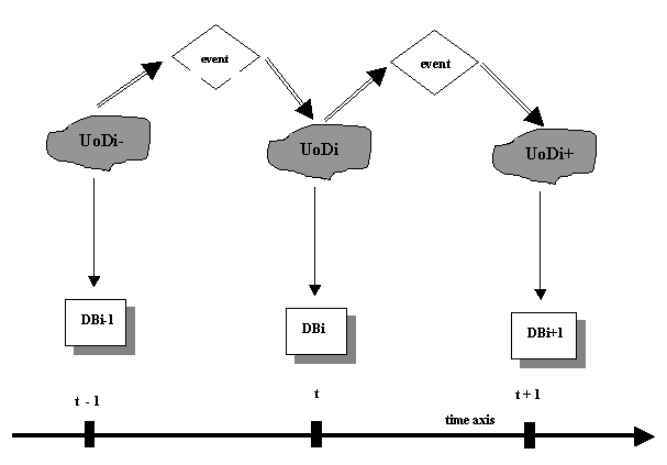
Figure 18.15
To give another example, assume that the UoD, and thus the database, contains information about employees and their salaries (see figure below). At time t-1 employee E1 has salary S1. At time t, the employee is given a salary increase and thus, his salary becomes S2. Later, at time t+1, the employee actually changes department and manager and his new salary becomes S3.
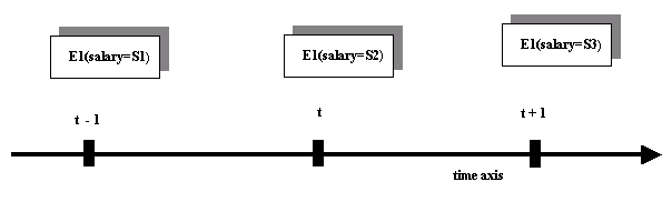
Figure 18.16
A temporal database is a database that deals with not only the ‘current’ state (in this example, t+1) but also with all the previous states of the salary history. To achieve that, we need to be able to model and reason about the time axis, and also be able to model and reason about the evolution of the data over time (usually referred to as the data or database history).
In order to deal with the time axis, the temporal database should have constructs to model the different notions of time (e.g. point, intervals, granularity and calendar units) and reason about them through temporal operators such as DURING and BEFORE. In the last two decades, the Relational data model has become the most popular database model because of its simplicity and solid mathematical foundation. However, the Relational data model originally proposed does not address the temporal dimension of data. Since there is a need for temporal data, many temporal extensions to Relational data models and query languages have been proposed. The incorporation of the temporal dimension has taken a number of different forms. One approach is the strategy of extending the schema of the relation to include one or more distinguished temporal attributes (e.g. START TIME, END TIME) to represent the intervals of time a tuple was ‘true’ for the database. This approach is called tuple timestamping. Another approach, referred to as attribute timestamping, involves adding additional attributes to the schema, with the domain of each attribute extended from simple values to complex values to incorporate the temporal dimension.
In this section we shall define some important concepts resulting from the previous discussions.
The valid time of a fact is the time when the fact is true in the modelled reality. A fact may have associated any number of instants and time intervals, with single instants and intervals being important special cases. Valid times are usually supplied by the user.
An example would be that Fred Bloggs was employed as marketing director at Matrix Incorporated from 1/3/1999 to 5/6/1999 — i.e. the valid time interval for a tuple recording that Fred Bloggs was marketing director is from 1/3/1999 to 5/6/1999.
The valid time has nothing to do with the time that data has been added to the database, so for example, we may have recorded this data and valid time about Fred Bloggs on 28/2/1999.
The valid time for data can be changed — e.g. perhaps Fred Bloggs comes out of retirement, and so a second interval from 12/10/2000 to 1/6/2001 is added to the valid times for his employment as marketing director.
A database fact is stored in a database at some point in time. A transaction time of a data fact is the time at which the information about a modelled object or event is stored in the database. The transaction time is automatically recorded by the DBMS and cannot be changed. If a fact is updated to a database at 10:15 on 4/2/1999, this transaction time never changes. If the data is changed at a later time, then a second transaction time is generated for the change, and so on. In this way a history of database changes based on transaction time timestamps is built up.
A timestamp is a time value associated with some object, e.g. an attribute value or a tuple. The concept may be specialised to valid timestamp, transaction timestamp or, for a particular temporal data model, some other kind of timestamp.
A calendar provides a human interpretation of time. As such, calendars ascribe meaning to temporal values where the particular meaning or interpretation is relevant to the user — in particular, the mapping between human-meaningful time values and underlying timeline. Calendars are most often cyclic, allowing human-meaningful time values to be expressed succinctly. For example, dates in the common Gregorian calendar may be expressed in the form <day, month, year> (for the UK) or <month, day, year> (for the US), where each of the fields 'day' and 'month' cycle as time passes (although year will continue to increase as time passes).
Different properties can be associated with a time axis composed from instants. Time is linear when the set of time points is completely ordered, also branching for the tasks of diagnosis, projection or forecasting (such as prediction of a medical evolution over time). Circular time describes recurrent events, such as "taking regular insulin every morning".
Review question 1
What are the differences between valid time and transaction time?
What are the differences between an absolute time and relative time? Give examples.
What are the differences between a time period and time interval? Give examples.
What are the differences between a time point and time period?
Four types of databases can be identified, according to the ability of a database to support valid time and/or transaction time, and the extent to which the database can be updated with regard to time.
A snapshot database can support either valid time or transaction time, but not both. It contains a ‘snapshot’ of the state of the database at a point in time. The term ‘snapshot’ is used to refer to the computational state of a database at a particular point in time.
If the data stored in the database represents a correct model of the world at this current point in time, then the database state represents transaction time — i.e. the database contents are the representation of the world for the current timestamp of the DBMS.
If the data stored in the database is valid or true at this current point in time, then the database state represents valid time.
Results from database operations take effect from commit time and past states are forgotten (overwritten). Snapshot databases are what one would usually think of as a database (with no recording of changes or past data values).
A rollback database has a sequence of states that are indexed by transaction time, i.e. the time the information was stored in the database. A rollback database preserves the past states of the database but not those of the real world. Therefore, it cannot correct errors in past information, nor represent that some facts will be valid for some future time.
Each time a change is made to a database, the before and after states are recorded for the transaction timestamp at the time the change takes place — so that at a later date, the database can be returned to a previous state.
These support only valid time. As defined earlier,valid time of a fact is the time when the fact is true in the modelled reality. The semantics of valid time are closely related to reality and, therefore, historical databases can maintain the history of the modelled Universe of Discourse and represent current knowledge about the past. However, historical databases cannot view the database as it was at some moment in the past.
In other words, a historical database can record that some fact F was valid from 1/1/1996 to 4/5/1998, but it is not recorded when these valid times were added to the database, so it is not possible to state that on 1/1/1997 it was recorded that fact F was true — perhaps we have retrospectively recorded when fact F was true at some time after 1/1/1997. Thus it is possible to reason about what we think was true for a given point of time, but not possible to answer questions about when we knew the facts were true, since no changes to the database have been recorded.
A historical database could be thought of as a snapshot of our beliefs about the past — at this point in time, we believe fact F was valid from 1/1/1996 to 4/5/1998 and that is all we can say.
These represent both transaction time and valid time and thus are both historical and rollback. So temporal databases record data about valid time (e.g. that we believe fact F is valid from 1/1/1996 to 4/5/1998) and the transaction time when such data was entered into the database (e.g. that we added this belief on 4/6/1997). This means that we can now rollback our temporal database to find out what our valid time beliefs were for any given past transaction time (e.g. what did we believe about fact F on 2/3/1997?).
Temporal databases allows retroactive update — i.e. coming into effect after the time to which the data was referenced. Temporal databases also support proactive update — i.e. coming into effect before the time to which the data was referenced. Thus, in a temporal database, we can represent explicitly a scenario such as the following:
Review question 2
What are the differences between relative and absolute times?
What are the differences between a snapshot database and a historical database?
What are the differences between a snapshot database and a temporal database?
In this final section, we briefly look at ways in which time data may be recorded and queried using extensions to the Relational model. It is not necessary to understand the fine details of temporal Relational query statements, but you should understand the different kinds of timestamping approaches, and the concepts around the two suggested temporal Relational operators, COALESCE and UNFOLD.
Let us now examine how the different types of temporal databases may be represented in the Relational model. A conventional relation can be visualised as a two-dimensional structure of tuples and attributes. Adding time as a third dimension to a conventional relation will change the relation into a three-dimensional structure. There have been many attempts in the past to find a suitable design structure that would be able to cope with handling the extra time dimension. We will describe these attempts in general, pointing out their successes and failures.
One of the earliest methods of maintaining time-based data for a database was to backup (archive) all the data stored in the database at regular intervals; i.e. the entire database was copied, with a timestamp, weekly or daily. However, information between backups is lost and retrieval of achieved information is slow and clumsy, since an entire version of the database needs to be loaded/searched.
The time-slicing method works if the database is stored as tables, such as in the Relational database model. When a change to the database occurs, at least one attribute of at least one tuple (record) from a particular table is changed. The time-slicing approach simply stores the entire table prior to the event and gives it a timestamp. Then a duplicate but updated copy is created and becomes part of the ‘live’ database state. Time-slicing is more efficient and easier to implement than archiving, since only those tables which are changed are copied with a timestamp. However, there still a lot of data redundancy in the time-slicing approach. This data redundancy is a result of duplicating a whole table when, for example, only one attribute value of one tuple was changed. With time-slicing, it is not possible to know the lifespan of a particular database state.
Tuple timestamping means that each relation is augmented with two time attributes representing a time interval, as illustrated in the figure below (the two attributes are the time points a tuple was ‘live’ for the database, i.e. starting time point and ending time point).
The entire table does not need to be duplicated; new tuples are simply added to the existing table when an event occurs. These new tuples are appended at the end of the table.
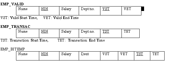
Figure 18.17
Examples:
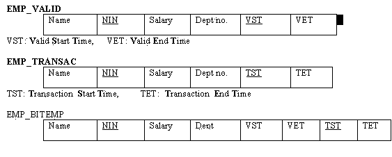
Figure 18.18
Example with data:
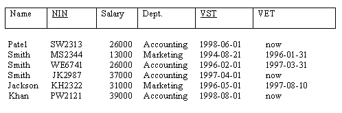
Figure 18.19
Attribute timestamping is implemented by attribute values consisting of two components, a timestamp and the data value. Some approaches to attribute timestamping use time intervals instead of timestamps, which express lifespan better than other constructs. Using time intervals can avoid the main problem of tuple timestamping, which breaks tuples into unmatched versions within or across tables. Retrieval is fast for single attributes, but poor for complete tuples.
The temporal Relational operators UNFOLD and COALESCE are important core concepts in most suggested extensions to the Relational model for temporal databases. The UNFOLD operator makes use of the concept of unary intervals introduced earlier in the chapter, and the COALECSE operator is the logical opposite of UNFOLD. We shall investigate each below.
The temporal Relational operator UNFOLD works on a set of tuples with valid or transaction time intervals (i.e. start and end time attributes) and expands the relation so that the data has a tuple for each unary interval appearing in any of the intervals for the data. This is probably best understood with an example. Consider the following temporal relation, NIGHTSHIFT, recording employees who are security guards for particular factory sites for particular dates (we will use valid dates in this example):
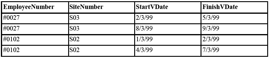
Figure 18.20
We can see intuitively from the table that employee #0027 has been on duty at site S03 for 2, 3, 4, 5 and 8, 9 March 1999. The UNFOLD operator makes this formal and explicit by replacing the tuples with intervals greater than one time quantum with multiple, unary intervals as follows:
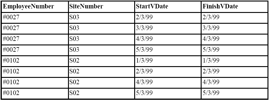
Figure 18.21
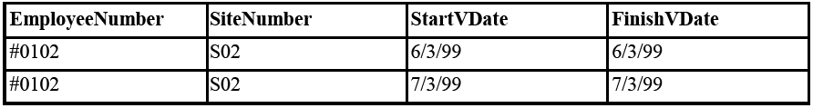
Figure 18.22
The usefulness of such an operator means that once a table has been UNFOLDED it becomes a simple query to find out whether a tuple was valid for any given time quantum.
The COALESCE temporal Relational operator is the logical opposite of UNFOLD in that it attempts to reduce the number of tuples to the minimum, i.e. wherever a sequence of intervals can be summarised in a single interval, this is done. Consider the following set of tuples for our NIGHTSHIFT relation:
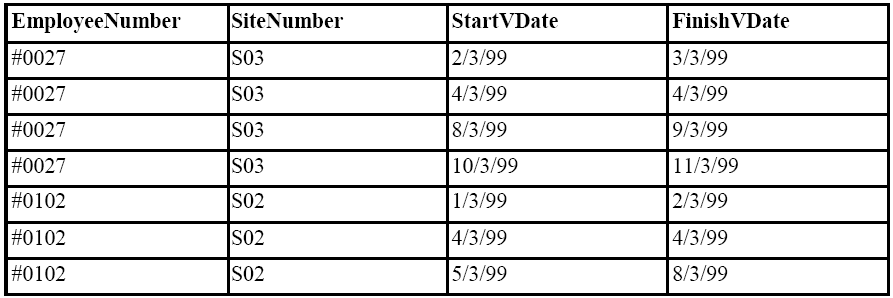
Figure 18.23
We might assume that employee #0027 came in for extras days on 4/3/99 to cover a colleague's sick leave; likewise for employee #0102 on 4/3/99.
We can see intuitively that employee #0027 was working from 2/3/99 until 4/3/99, and from 8/3/99 until 11/3/99. The COALESCE temporal Relational operator formalises this concept of using the minimum number of tuples to represent the intervals when data is valid. The result of the COALESCE query on the relation is as follows:
Result of query: NIGHTSHIFT COALESCE StartVDate, FinishVDate
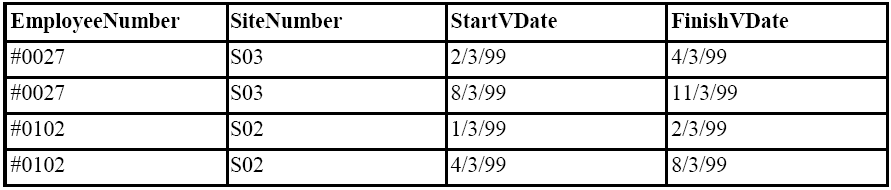
Figure 18.24
You may wish to refer to the recommended reading for this chapter to investigate further the details of these two temporal Relational operators.
Consider the following statements spoken in 2015.
"Two days ago, I was seven years old," said a little girl. "Next year, I'll be 10!"
Can this be true? If so, what was the date the little girl was born, and what was the date when she was speaking?
Discuss how time instants and time periods can be use to model time-oriented medical data.
Amongst many existing data models, we have chosen the Entity Relationship Time (ERT) model for its simplicity and the support of the SQL language.
The Entity Relationship Time model (ERT) is an extended entity-relationship type model that additionally accommodates 'complex objects' and 'time'. The ERT model consists of the following concepts:
Entity: Anything, concrete or abstract, uniquely identifiable and being of interest during a certain time period.
Entity class: The collection of all the entities to which a specific definition and common properties apply at a specific time period.
Relationship: Any permanent or temporary association between two entities or between an entity and a value.
Relationship class: The collection of all the relationships to which a specific definition applies at a specific time period.
Value: An object perceived individually, which is only of interest when it is associated with an entity. That is, values cannot exist on their own.
Value class: The proposition establishing a domain of values.
Time period: A pair of time points expressed at the same abstraction level.
Time period class: A collection of time periods.
Complex object: A complex value or a complex entity. A complex entity is an abstraction (aggregation or grouping) of entities and relationships. A complex value is an abstraction (aggregation or grouping) of simple values.
Complex object class: A collection of complex objects. That is, it can be a complex entity or a complex value class.
The time structure denotes the granularity of the timestamp. Various types of granularity are provided including: second, minute, hour, day, month and year. The default granularity type is the second. Obviously, if the user specifies a granularity type for a timestamped ERT object, this granularity type supports all the super types of it. For example, if the day granularity type is specified, the actual timestamp values will have a year, a month and a day reference. Furthermore, the time structure can be user-defined, e.g. a granularity of a week may be necessary.
Besides the temporal dimension, ERT differs from the entity-relationship model in that it regards any association between objects as the unified form of a relationship, thus avoiding the unnecessary distinction between attributes and relationships. A relationship class denotes a set of associations between two entity classes or between an entity class and a value class, and in that, all relationships are binary and each relationship has its inverse. Additionally, for every relationship class, apart from the objects participating, the relationship involvements of the objects and the cardinality constraints should be specified.
The relationship involvements specify the roles of the object in the specified relationship e.g. Employee works_for Department, Department employs Employee. Furthermore, for each relationship involvement, a user-supplied constraint rule must be defined which restricts the number of times an entity or a value can participate in this involvement. This constraint is called a cardinality constraint and it is applied to the instances of the relationship by restricting its population. As an example, consider the case where the constraint for relationship (Employee, works_for, Department) is 1:N. This is interpreted as: one Employee can be associated to at least one instance of Department, while there is no upper limit to the number of Departments an Employee is associated with.
Another additional feature of the ERT model is the concept of complex object (entity or value class). The basic motivation for the inclusion of the complex object class in the external formalism, is to abstract away detail, which in several cases is not of interest. In addition, no distinction is made between aggregation and grouping, but rather a general composition mechanism is considered which involves relationships/attributes. For the modelling of complex objects, a special type of relationship class is provided, named IsPartOf.
An entity or relationship class can be derived. This implies that its instances are not stored by default, but for each such derivable component, there is a corresponding derivation rule which gives the instances of this class at any time. Derived schema components are one of the fundamental mechanisms in semantic models for data abstraction and encapsulation.
The graphical representation of ERT constructs is depicted below.
The construct of timestamp is modelled as a pair (a,b), where a denotes the temporal semantic category (TSC) while b denotes the time structure. Three different temporal semantic categories have been identified, namely:
Decomposable
Nondecomposable
time points
The ERT notation for the three concepts is TPI for the decomposable time periods, TI for the nondecomposable time interval and TP for the time point. The time structure denotes the granularity of the timestamp.
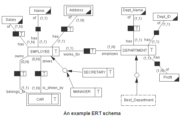
Figure 18.25
An example ERT schema is depicted in the figure above. Several entity classes can be found in the diagram, namely: Employee, Manager, Secretary, Department and Car. These are represented using a rectangle with the addition of a ‘time box’, which shows that the entity is time varying. Complex entity classes are represented using double rectangles, e.g. Car, while for derived entity class the rectangle is dashed, e.g. Best_Department. For the entity classes participating in a hierarchy, an arrow is used for specifying the parent entity class.
Relationship classes are represented using a small filled rectangle and can be time varying (with the addition of ‘T’) or not. In addition, for every relationship class, relationship involvements and cardinality constraints are specified.
Value classes e.g. Name, Address or Dept_ID, are represented with rectangles which have a small black triangle at the bottom right corner. Complex value classes e.g. Address are represented using double rectangles.
Every complex object can be further analysed into its components. The notation used is the same as in the top-level schema, adding the special type relationship IsPartOf. The complex entity class Car is illustrated in the first figure below, while the complex value class Address is illustrated in the second figure below.
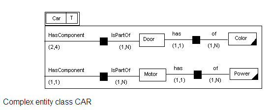
Figure 18.26
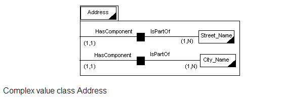
Figure 18.27
An example of a derived entity class is illustrated in the figure below, and population of entity class Employee and entity class Department are shown in the two tables below that.
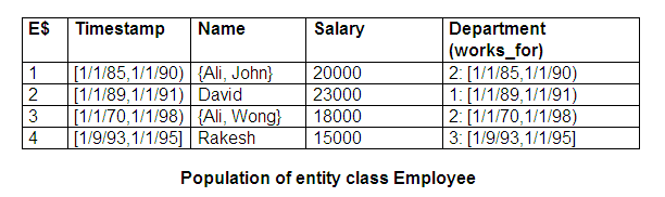
Figure 18.28
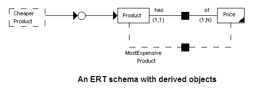
Figure 18.29
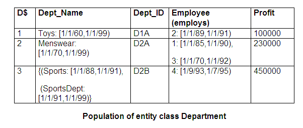
Figure 18.30
In this section, we describe the temporal query language ERT-SQL primarily used for manipulating an ERT-based database. The ERT-SQL is based on the standard SQL2 and on the valid time SQL (VT-SQL) language.
The ERT-SQL statements are divided into three language groups:
Data Definition Language (DDL): These statements are used to define the ERT schema, by specifying one by one all ERT components (for example, CREATE ENTITY, CREATE RELATIONSHIP).
Data Manipulation Language (DML): DML statements are used to query or update data of an ERT database (for example, SELECT, INSERT).
Schema Manipulation Language (SML): These statements are used to alter the ERT schema (for example DROP ENTITY, ALTER ENTITY).
Full description of ERT-SQL is beyond the scope of this chapter. Thus, in the rest of this section, the capabilities of ERT-SQL are illustrated with a number of examples.
The CREATE statement has the structure and facilities similar to that of the standard SQL, but it is extended in order to be able to capture the temporal and structural semantics of the ERT model.
“Create entity employee class, employee and also relationship class (employee, department).”
CREATE ENTITY Employee (TPI,DAY )
(VALUE,Name,CHAR(20),has,1,1,of,1,1)
(VALUE,Salary,INTEGER,has,1,N,of,1,N(TPI,DAY))
(COMPLEX VALUE,Address,has,1,1,of,1,N(TPI,DAY))
CREATE RELATIONSHIP (Employee,Department,works_for,1,1,employs,1,N(TI,MONTH))
The SELECT statement also has the structure and facilities similar to that of the standard, with temporal capability.
"Give the periods during which the employee 'Ali' had been working for the 'Toys' department.”
SELECT [Employee, Department, works_for].TIMESTAMP
FROM Employee, Department
WHERE Dept_Name = 'Toys' AND Name='Ali'
The INSERT statement is used to add instances both to entity and to relationship classes.
“Insert the 'Toys' department with existence period from the first day of 1994 and Profit £10000.”
INSERT INTO Department
VALUES
Dept_ID = 'D151294'
Dept_Name = 'Toys' '[1/1/1994, )'
Profit = 10000
TIMESTAMP = '[1/1/1994, )'
“Insert the information that the employee with name 'Ali' has been working for the 'Toys' department from 5/4/1994 to 1/5/1996.”
INSERT INTO RELATIONSHIP (Employee, Department, works_for)
TIMESTAMP = '[5/4/1994, 1/5/1996)'
WHERE (Name = ('Ali')) AND (Dept_Name = 'Toys')
The DELETE statement is used to delete particular instances from an entity class or from a relationship class.
"Delete the information that the employee 'Ali' had worked for the 'Toys' department for the period [1/1/1990,1/2/1990)."
DELETE FROM RELATIONSHIP (Employee,Department,works_for)
WHERE ( TIMESTAMP = '[1/1/1990, 1/2/1990)') AND (Name = 'Ali') AND (Dept_Name = 'Toys')
The UPDATE statement is used to alter the contents of an instance either of an entity class or of a relationship class.
"The department 'Toys' had this name for the period '[1/1/1970,1/1/1987)' and not for the '[1/1/1960,1/1/1990)'. Enter the correct period."
UPDATE RELATIONSHIP( Department, Dept_Name, has )
SET TIMESTAMP = '[1/1/1970,1/1/1987)'
WHERE(TIMESTAMP='[1/1/1960,1/1/1990)') AND (Dept_Name='Toys')
The DROP statement is used to remove entity classes (simple, complex or derived) or relationship classes from an ERT schema.
"Remove the Department entity class."
DROP ENTITY Department
"Remove the relationship class between entities Employee and Car with role name 'owns'."
DROP RELATIONSHIP (Employee, Car, owns)
The ALTER statement is used to add and remove value classes or to add a new component to a complex object.
"Add to the entity Employee, value class 'Bank_Account'."
ALTER ENTITY Employee
ADD (VALUE,Bank_Account,INTEGER,has,1,1,of,1,N)
“Alter timestamped relationship between Employee and Department. Set temporal semantic category to TPI and granularity to DAY.”
ALTER RELATIONSHIP
(Employee, Department, works_for)
TIMESTAMP (TPI,DAY)
Additional review questions
“Insert the information that the employee with name 'Ali' has been working for the 'Toys' department from 5/4/1994 to 1/5/1996.”
“Alter timestamped relationship between Employee and Department. Set temporal semantic category to TPI and granularity to DAY.”