Figure 19.1
Table of contents
At the end of this chapter you should be able to:
Distinguish a data warehouse from an operational database system, and appreciate the need for developing a data warehouse for large corporations.
Describe the problems and processes involved in the development of a data warehouse.
Explain the process of data mining and its importance.
Understand different data mining techniques.
Rapid developments in information technology have resulted in the construction of many business application systems in numerous areas. Within these systems, databases often play an essential role. Data has become a critical resource in many organisations, and therefore, efficient access to the data, sharing the data, extracting information from the data, and making use of the information stored, has become an urgent need. As a result, there have been many efforts on firstly integrating the various data sources (e.g. databases) scattered across different sites to build a corporate data warehouse, and then extracting information from the warehouse in the form of patterns and trends.
A data warehouse is very much like a database system, but there are distinctions between these two types of systems. A data warehouse brings together the essential data from the underlying heterogeneous databases, so that a user only needs to make queries to the warehouse instead of accessing individual databases. The co-operation of several processing modules to process a complex query is hidden from the user.
Essentially, a data warehouse is built to provide decision support functions for an enterprise or an organisation. For example, while the individual data sources may have the raw data, the data warehouse will have correlated data, summary reports, and aggregate functions applied to the raw data. Thus, the warehouse is able to provide useful information that cannot be obtained from any individual databases. The differences between the data warehousing system and operational databases are discussed later in the chapter.
We will also see what a data warehouse looks like – its architecture and other design issues will be studied. Important issues include the role of metadata as well as various access tools. Data warehouse development issues are discussed with an emphasis on data transformation and data cleansing. Star schema, a popular data modelling approach, is introduced. A brief analysis of the relationships between database, data warehouse and data mining leads us to the second part of this chapter - data mining.
Data mining is a process of extracting information and patterns, which are previously unknown, from large quantities of data using various techniques ranging from machine learning to statistical methods. Data could have been stored in files, Relational or OO databases, or data warehouses. In this chapter, we will introduce basic data mining concepts and describe the data mining process with an emphasis on data preparation. We will also study a number of data mining techniques, including decision trees and neural networks.
We will also study the basic concepts, principles and theories of data warehousing and data mining techniques, followed by detailed discussions. Both theoretical and practical issues are covered. As this is a relatively new and popular topic in databases, you will be expected to do some extensive searching, reading and discussion during the process of studying this chapter.
In parallel with this chapter, you should read Chapter 31, Chapter 32 and Chapter 34 of Thomas Connolly and Carolyn Begg, "Database Systems A Practical Approach to Design, Implementation, and Management", (5th edn.).
A data warehouse is an environment, not a product. The motivation for building a data warehouse is that corporate data is often scattered across different databases and possibly in different formats. In order to obtain a complete piece of information, it is necessary to access these heterogeneous databases, obtain bits and pieces of partial information from each of them, and then put together the bits and pieces to produce an overall picture. Obviously, this approach (without a data warehouse) is cumbersome, inefficient, ineffective, error-prone, and usually involves huge efforts of system analysts. All these difficulties deter the effective use of complex corporate data, which usually represents a valuable resource of an organisation.
In order to overcome these problems, it is considered necessary to have an environment that can bring together the essential data from the underlying heterogeneous databases. In addition, the environment should also provide facilities for users to carry out queries on all the data without worrying where it actually resides. Such an environment is called a data warehouse. All queries are issued to the data warehouse as if it is a single database, and the warehouse management system will handle the evaluation of the queries.
Different techniques are used in data warehouses, all aimed at effective integration of operational databases into an environment that enables strategic use of data. These techniques include Relational and multidimensional database management systems, client-server architecture, metadata modelling and repositories, graphical user interfaces, and much more.
A data warehouse system has the following characteristics:
It provides a centralised utility of corporate data or information assets.
It is contained in a well-managed environment.
It has consistent and repeatable processes defined for loading operational data.
It is built on an open and scalable architecture that will handle future expansion of data.
It provides tools that allow its users to effectively process the data into information without a high degree of technical support.
A data warehouse is conceptually similar to a traditional centralised warehouse of products within the manufacturing industry. For example, a manufacturing company may have a number of plants and a centralised warehouse. Different plants use different raw materials and manufacturing processes to manufacture goods. The finished products from the plants will then be transferred to and stored in the warehouse. Any queries and deliveries will only be made to and from the warehouse rather than the individual plants.
Using the above analogy, we can say that a data warehouse is a centralised place to store data (i.e. the finished products) generated from different operational systems (i.e. plants). For a big corporation, for example, there are normally a number of different departments/divisions, each of which may have its own operational system (e.g. database). These operational systems generate data day in and day out, and the output from these individual systems can be transferred to the data warehouse for further use. Such a transfer, however, is not just a simple process of moving data from one place to another. It is a process involving data transformation and possibly other operations as well. The purpose is to ensure that heterogeneous data will conform to the same specification and requirement of the data warehouse.
Building data warehouses has become a rapidly expanding requirement for most information technology departments. The reason for growth in this area stems from many places:
With regard to data, most companies now have access to more than 20 years of data on managing the operational aspects of their business.
With regard to user tools, the technology of user computing has reached a point where corporations can now effectively allow the users to navigate corporation databases without causing a heavy burden to technical support.
With regard to corporate management, executives are realising that the only way to sustain and gain an advantage in today’s economy is to better leverage information.
Before we proceed to detailed discussions of data warehousing systems, it is beneficial to note some of the major differences between operational and data warehousing systems.
Operational systems are those that assist a company or an organisation in its day-to-day business to respond to events or transactions. As a result, operational system applications and their data are highly structured around the events they manage. These systems provide an immediate focus on business functions and typically run in an online transaction processing (OLTP) computing environment. The databases associated with these applications are required to support a large number of transactions on a daily basis. Typically, operational databases are required to work as fast as possible. Strategies for increasing performance include keeping these operational data stores small, focusing the database on a specific business area or application, and eliminating database overhead in areas such as indexes.
Operational system applications and their data are highly structured around the events they manage. Data warehouse systems are organised around the trends or patterns in those events. Operational systems manage events and transactions in a similar fashion to manual systems utilised by clerks within a business. These systems are developed to deal with individual transactions according to the established business rules. Data warehouse systems focus on business needs and requirements that are established by managers, who need to reflect on events and develop ideas for changing the business rules to make these events more effective.
Operational systems and data warehouses provide separate data stores. A data warehouse’s data store is designed to support queries and applications for decision-making. The separation of a data warehouse and operational systems serves multiple purposes:
It minimises the impact of reporting and complex query processing on operational systems.
It preserves operational data for reuse after that data has been purged from the operational systems.
It manages the data based on time, allowing the user to look back and see how the company looked in the past versus the present.
It provides a data store that can be modified to conform to the way the users view the data.
It unifies the data within a common business definition, offering one version of reality.
A data warehouse assists a company in analysing its business over time. Users of data warehouse systems can analyse data to spot trends, determine problems and compare business techniques in a historical context. The processing that these systems support include complex queries, ad hoc reporting and static reporting (such as the standard monthly reports that are distributed to managers). The data that is queried tends to be of historical significance and provides its users with a time-based context of business processes.
While a company can better manage its primary business with operational systems through techniques that focus on cost reduction, data warehouse systems allow a company to identify opportunities for increasing revenues, and therefore, for growing the business. From a business point of view, this is the primary way to differentiate these two mission-critical systems. However, there are many other key differences between these two types of systems.
Size and content: The goals and objectives of a data warehouse differ greatly from an operational environment. While the goal of an operational database is to stay small, a data warehouse is expected to grow large – to contain a good history of the business. The information required to assist us in better understanding our business can grow quite voluminous over time, and we do not want to lose this data.
Performance: In an operational environment, speed is of the essence. However, in a data warehouse, some requests – 'meaning-of-life' queries – can take hours to fulfil. This may be acceptable in a data warehouse environment, because the true goal is to provide better information, or business intelligence. For these types of queries, users are typically given a personalised extract of the requested data so they can further analyse and query the information package provided by the data warehouse.
Content focus: Operational systems tend to focus on small work areas, not the entire enterprise; a data warehouse, on the other hand, focuses on cross-functional subject areas. For example, a data warehouse could help a business understand who its top 20 at-risk customers are – those who are about to drop their services – and what type of promotions will assist in not losing these customers. To fulfil this query request, the data warehouse needs data from the customer service application, the sales application, the order management application, the credit application and the quality system.
Tools: Operational systems are typically structured, offering only a few ways to enter or access the data that they manage, and lack a large amount of tools accessibility for users. A data warehouse is the land of user tools. Various tools are available to support the types of data requests discussed earlier. These tools provide many features that transform and present the data from a data warehouse as business intelligence. These features offer a high flexibility over the standard reporting tools that are offered within an operational systems environment.
Driven by the need to gain competitive advantage in the marketplace, organisations are now seeking to convert their operational data into useful business intelligence – in essence fulfilling user information requirements. The user’s questioning process is not as simple as one question and the resultant answer. Typically, the answer to one question leads to one or more additional questions. The data warehousing systems of today require support for dynamic iterative analysis – delivering answers in a rapid fashion. Data warehouse systems, often characterised by query processing, can assist in the following areas:
Consistent and quality data: For example, a hospital system had a severe data quality problem within its operational system that captured information about people serviced. The hospital needed to log all people who came through its door regardless of the data that was provided. This meant that someone who checked in with a gunshot wound and told the staff his name was Bob Jones, and who subsequently lost consciousness, would be logged into the system identified as Bob Jones. This posed a huge data quality problem, because Bob Jones could have been Robert Jones, Bobby Jones or James Robert Jones. There was no way of distinguishing who this person was. You may be saying to yourself, big deal! But if you look at what a hospital must do to assist a patient with the best care, this is a problem. What if Bob Jones were allergic to some medication required to treat the gunshot wound? From a business sense, who was going to pay for Bob Jones' bills? From a moral sense, who should be contacted regarding Bob Jones’ ultimate outcome? All of these directives had driven this institution to a proper conclusion: They needed a data warehouse. This information base, which they called a clinical repository, would contain quality data on the people involved with the institution – that is, a master people database. This data source could then assist the staff in analysing data as well as improving the data capture, or operational system, in improving the quality of data entry. Now when Bob Jones checks in, they are prompted with all of the patients called Bob Jones who have been treated. The person entering the data is presented with a list of valid Bob Joneses and several questions that allow the staff to better match the person to someone who was previously treated by the hospital.
Cost reduction: Monthly reports produced by an operational system could be expensive to store and distribute. In addition, very little content in the reports is typically universally useful, and because the data takes so long to produce and distribute, it's out of sync with the users' requirements. A data warehouse implementation can solve this problem. We can index the paper reports online and allow users to select the pages of importance to be loaded electronically to the users’ personal workstations. We could save a bundle of money just by eliminating the distribution of massive paper reports.
More timely data access: As noted earlier, reporting systems have become so unwieldy that the data they present is typically unusable after it is placed in users’ hands. What good is a monthly report if you do not get it until the end of the following month? How can you change what you are doing based on data that old? The reporting backlog has never dissipated within information system departments; typically it has grown. Granting users access to data on a more timely basis allows them to better perform their business tasks. It can also assist in reducing the reporting backlog, because users take more responsibility for the reporting process.
Improved performance and productivity: Removing information systems professionals from the reporting loop and empowering users results in internal efficiency. Imagine that you had no operational systems and had to hunt down the person who recorded a transaction to better understand how to improve the business process or determine whether a promotion was successful. The truth is that all we have done is automate this nightmare with the current operational systems. Users have no central sources for information and must search all of the operational systems for the data that is required to answer their questions. A data warehouse assists in eliminating information backlogs, reporting backlogs, information system performance problems and so on by improving the efficiency of the process, eliminating much of the information search missions.
It should be noted that even with a data warehouse, companies still require two distinct kinds of reporting: that which provides notification of operational conditions needing response, and that which provides general information, often summarised, about business operations. The notification-style reports should still be derived from operational systems, because detecting and reporting these conditions is part of the process of responding to business events. The general information reports, indicating operational performance typically used in analysing the business, are managed by a data warehouse.
Review question 1
Analyse the differences between data warehousing and operational systems, and discuss the importance of the separation of the two systems.
Activity 1
Research how a business in your area of interest has benefited from the data warehousing technology.
Data warehouses provide a means to make information available for decision-making. An effective data warehousing strategy must deal with the complexities of modern enterprises. Data is generated everywhere, and controlled by different operational systems and data storage mechanisms. Users demand access to data anywhere and any time, and data must be customised to their needs and requirements. The function of a data warehouse is to prepare the current transactions from operational systems into data with a historical context, required by the users of the data warehouse.
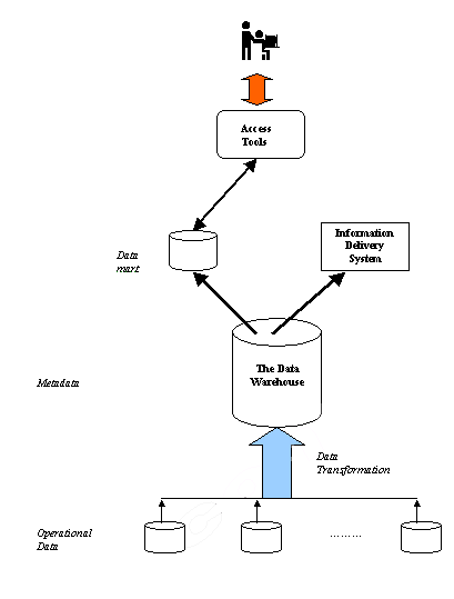
The general data warehouse architecture is based on a Relational database management system server that functions as the central repository for informational data. In the data warehouse architecture, operational data and processing is completely separate from data warehouse processing. This central information repository is surrounded by a number of key components designed to make the entire environment functional, manageable and accessible by both the operational systems that source data into the warehouse and by end-user query and analysis tools. The diagram below depicts such a general architecture:
Figure 19.1
Typically, the source data for the warehouse is coming from the operational applications, or an operational data store (ODS). As the data enters the data warehouse, it is transformed into an integrated structure and format. The transformation process may involve conversion, summarisation, filtering and condensation of data. Because data within the data warehouse contains a large historical component (sometimes over 5 to 10 years), the data warehouse must be capable of holding and managing large volumes of data as well as different data structures for the same database over time.
The central data warehouse database is a cornerstone of the data warehousing environment. This type of database is mostly implemented using a Relational DBMS (RDBMS). However, a warehouse implementation based on traditional RDBMS technology is often constrained by the fact that traditional RDBMS implementations are optimised for transactional database processing. Certain data warehouse attributes, such as very large database size, ad hoc query processing and the need for flexible user view creation, including aggregates, multi-table joins and drill-downs, have become drivers for different technological approaches to the data warehouse database.
A significant portion of the data warehouse implementation effort is spent extracting data from operational systems and putting it in a format suitable for information applications that will run off the data warehouse. The data-sourcing, clean-up, transformation and migration tools perform all of the conversions, summarisation, key changes, structural changes and condensations needed to transform disparate data into information that can be used by the decision support tool. It also maintains the metadata. The functionality of data transformation includes:
Removing unwanted data from operational databases.
Converting to common data names and definitions.
Calculating summaries and derived data.
Establishing defaults for missing data.
Accommodating source data definition changes.
The data-sourcing, clean-up, extraction, transformation and migration tools have to deal with some important issues as follows:
Database heterogeneity: DBMSs can vary in data models, data access languages, data navigation operations, concurrency, integrity, recovery, etc.
Data heterogeneity: This is the difference in the way data is defined and used in different models – there are homonyms, synonyms, unit incompatibility, different attributes for the same entity, and different ways of modelling the same fact.
A crucial area of data warehousing is metadata, which is a kind of data that describes the data warehouse itself. Within a data warehouse, metadata describes and locates data components, their origins (which may be either the operational systems or the data warehouse), and their movement through the data warehouse process. The data access, data stores and processing information will have associated descriptions about the data and processing – the inputs, calculations and outputs – documented in the metadata. This metadata should be captured within the data architecture and managed from the beginning of a data warehouse project. The metadata repository should contain information such as that listed below:
Description of the data model.
Description of the layouts used in the database design.
Definition of the primary system managing the data items.
A map of the data from the system of record to the other locations in the data warehouse, including the descriptions of transformations and aggregations.
Specific database design definitions.
Data element definitions, including rules for derivations and summaries.
It is through metadata that a data warehouse becomes an effective tool for an overall enterprise. This repository of information will tell the story of the data: where it originated, how it has been transformed, where it went and how often – that is, its genealogy or artefacts. Technically, the metadata will also improve the maintainability and manageability of a warehouse by making impact analysis information and entity life histories available to the support staff.
Equally important, metadata provides interactive access to users to help understand content and find data. Thus, there is a need to create a metadata interface for users.
One important functional component of the metadata repository is the information directory. The content of the information directory is the metadata that helps users exploit the power of data warehousing. This directory helps integrate, maintain and view the contents of the data warehousing system. From a technical requirements point of view, the information directory and the entire metadata repository should:
Be a gateway to the data warehouse environment, and therefore, should be accessible from any platform via transparent and seamless connections.
Support an easy distribution and replication of its content for high performance and availability.
Be searchable by business-oriented keywords.
Act as a launch platform for end-user data access and analysis tools.
Support the sharing of information objects such as queries, reports, data collections and subscriptions between users.
Support a variety of scheduling options for requests against the data warehouse, including on-demand, one-time, repetitive, event-driven and conditional delivery (in conjunction with the information delivery system).
Support the distribution of query results to one or more destinations in any of the user-specified formats (in conjunction with the information delivery system).
Support and provide interfaces to other applications such as e-mail, spreadsheet and schedules.
Support end-user monitoring of the status of the data warehouse environment.
At a minimum, the information directory components should be accessible by any Web browser, and should run on all major platforms, including MS Windows, Windows NT and UNIX. Also, the data structures of the metadata repository should be supported on all major Relational database platforms.
These requirements define a very sophisticated repository of metadata information. In reality, however, existing products often come up short when implementing these requirements.
The principal purpose of data warehousing is to provide information to business users for strategic decision-making. These users interact with the data warehouse using front-end tools. Although ad hoc requests, regular reports and custom applications are the primary delivery vehicles for the analysis done in most data warehouses, many development efforts of data warehousing projects are focusing on exceptional reporting also known as alerts, which alert a user when a certain event has occurred. For example, if a data warehouse is designed to access the risk of currency trading, an alert can be activated when a certain currency rate drops below a predefined threshold. When an alert is well synchronised with the key objectives of the business, it can provide warehouse users with a tremendous advantage.
The front-end user tools can be divided into five major groups:
Data query and reporting tools.
Application development tools.
Executive information systems (EIS) tools.
Online analytical processing (OLAP) tools.
Data mining tools.
This category can be further divided into two groups: reporting tools and managed query tools. Reporting tools can be divided into production reporting tools and desktop report writers.
Production reporting tools let companies generate regular operational reports or support high-volume batch jobs, such as calculating and printing pay cheques. Report writers, on the other hand, are affordable desktop tools designed for end-users.
Managed query tools shield end-users from the complexities of SQL and database structures by inserting a metalayer between users and the database. The metalayer is the software that provides subject-oriented views of a database and supports point-and-click creation of SQL. Some of these tools proceed to format the retrieved data into easy-to-read reports, while others concentrate on on-screen presentations. These tools are the preferred choice of the users of business applications such as segment identification, demographic analysis, territory management and customer mailing lists. As the complexity of the questions grows, these tools may rapidly become inefficient.
Often, the analytical needs of the data warehouse user community exceed the built-in capabilities of query and reporting tools. Organisations will often rely on a true and proven approach of in-house application development, using graphical data access environments designed primarily for client-server environments. Some of these application development platforms integrate well with popular OLAP tools, and can access all major database systems, including Oracle and IBM Informix.
The target users of EIS tools are senior management of a company. The tools are used to transform information and present that information to users in a meaningful and usable manner. They support advanced analytical techniques and free-form data exploration, allowing users to easily transform data into information. EIS tools tend to give their users a high-level summarisation of key performance measures to support decision-making.
These tools are based on concepts of multidimensional database and allow a sophisticated user to analyse the data using elaborate, multidimensional and complex views. Typical business applications for these tools include product performance and profitability, effectiveness of a sales program or a marketing campaign, sales forecasting and capacity planning. These tools assume that the data is organised in a multidimensional model, which is supported by a special multidimensional database or by a Relational database designed to enable multidimensional properties.
Data mining can be defined as the process of discovering meaningful new correlation, patterns and trends by digging (mining) large amounts of data stored in a warehouse, using artificial intelligence (AI) and/or statistical/mathematical techniques. The major attraction of data mining is its ability to build predictive rather than retrospective models. Using data mining to build predictive models for decision-making has several benefits. First, the model should be able to explain why a particular decision was made. Second, adjusting a model on the basis of feedback from future decisions will lead to experience accumulation and true organisational learning. Finally, a predictive model can be used to automate a decision step in a larger process. For example, using a model to instantly predict whether a customer will default on credit card payments will allow automatic adjustment of credit limits rather than depending on expensive staff making inconsistent decisions. Data mining will be discussed in more detail later on in the chapter.
Data warehouses are causing a surge in popularity of data visualisation techniques for looking at data. Data visualisation is not a separate class of tools; rather, it is a method of presenting the output of all the previously mentioned tools in such a way that the entire problem and/or the solution (e.g. a result of a Relational or multidimensional query, or the result of data mining) is clearly visible to domain experts and even casual observers.
Data visualisation goes far beyond simple bar and pie charts. It is a collection of complex techniques that currently represent an area of intense research and development, focusing on determining how to best display complex relationships and patterns on a two-dimensional (flat) computer monitor. Similar to medical imaging research, current data visualisation techniques experiment with various colours, shapes, 3D imaging and sound, and virtual reality to help users really see and feel the problem and its solutions.
The concept of data mart is causing a lot of excitement and attracts much attention in the data warehouse industry. Mostly, data marts are presented as an inexpensive alternative to a data warehouse that takes significantly less time and money to build. However, the term means different things to different people. A rigorous definition of data mart is that it is a data store that is subsidiary to a data warehouse of integrated data. The data mart is directed at a partition of data (often called subject area) that is created for the use of a dedicated group of users. A data mart could be a set of denormalised, summarised or aggregated data. Sometimes, such a set could be placed on the data warehouse database rather than a physically separate store of data. In most instances, however, a data mart is a physically separate store of data and is normally resident on a separate database server, often on the local area network serving a dedicated user group.
Data marts can incorporate different techniques like OLAP or data mining. All these types of data marts are called dependent data marts because their data content is sourced from the data warehouse. No matter how many are deployed and what different enabling technologies are used, different users are all accessing the information views derived from the same single integrated version of the data (i.e. the underlying warehouse).
Unfortunately, the misleading statements about the simplicity and low cost of data marts sometimes result in organisations or vendors incorrectly positioning them as an alternative to the data warehouse. This viewpoint defines independent data marts that in fact represent fragmented point solutions to a range of business problems. It is missing the integration that is at the heart of the data warehousing concept: data integration. Each independent data mart makes its own assumptions about how to consolidate data, and as a result, data across several data marts may not be consistent.
Moreover, the concept of an independent data mart is dangerous – as soon as the first data mart is created, other organisations, groups and subject areas within the enterprise embark on the task of building their own data marts. As a result, you create an environment in which multiple operational systems feed multiple non-integrated data marts that are often overlapping in data content, job scheduling, connectivity and management. In other words, you have transformed a complex many-to-one problem of building a data warehouse from operational data sources into a many-to-many sourcing and management nightmare. Another consideration against independent data marts is related to the potential scalability problem.
To address data integration issues associated with data marts, a commonly recommended approach is as follows. For any two data marts in an enterprise, the common dimensions must conform to the equality and roll-up rule, which states that these dimensions are either the same or that one is a strict roll-up of another.
Thus, in a retail store chain, if the purchase orders database is one data mart and the sales database is another data mart, the two data marts will form a coherent part of an overall enterprise data warehouse if their common dimensions (e.g. time and product) conform. The time dimension from both data marts might be at the individual day level, or conversely, one time dimension is at the day level but the other is at the week level. Because days roll up to weeks, the two time dimensions are conformed. The time dimensions would not be conformed if one time dimension were weeks and the other a fiscal quarter. The resulting data marts could not usefully coexist in the same application.
The key to a successful data mart strategy is the development of an overall scalable data warehouse architecture, and the key step in that architecture is identifying and implementing the common dimensions.
The information delivery system distributes warehouse-stored data and other information objects to other data warehouses and end-user products such as spreadsheets and local databases. Delivery of information may be based on time of day, or on the completion of an external event. The rationale for the delivery system component is based on the fact that once the data warehouse is installed and operational, its users don’t have to be aware of its location and maintenance. All they may need is the report or an analytical view of data, at a certain time of the day, or based on a particular, relevant event. And of course, such a delivery system may deliver warehouse-based information to end users via the Internet. A Web-enabled information delivery system allows users dispersed across continents to perform sophisticated business-critical analysis, and to engage in collective decision-making that is based on timely and valid information.
Review question 2
Discuss the functionality of data transformation in a data warehouse system.
What is metadata? How is it used in a data warehouse system?
What is a data mart? What are the drawbacks of using independent data marts?
A data warehouse blueprint should include clear documentation of the following items:
Requirements: What does the business want from the data warehouse?
Architecture blueprint: How will you deliver what the business wants?
Development approach: What is a clear definition of phased delivery cycles, including architectural review and refinement processes?
The blueprint document essentially translates an enterprise’s mission, goals and objectives for the data warehouse into a logical technology architecture composed of individual sub-architectures for the application, data and technology components of a data warehouse, as shown below:
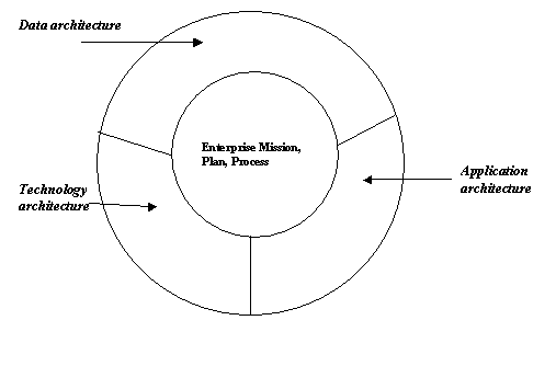
Figure 19.2
An architecture blueprint is important, because it serves as a road map for all development work and as a guide for integrating the data warehouse with legacy systems. When the blueprint is understood by the development staff, decisions become much easier. The blueprint should be developed in a logical sense rather than in a physical sense. For the database components, for example, you will state things like “the data store for the data warehouse will support an easy-to-use data manipulation language that is standard in the industry, such as SQL”. This is a logical architecture-product requirement. When you implement the data warehouse, this could be Sybase SQL Server or Oracle. The logical definition allows your implementations to grow as technology evolves. If your business requirements do not change in the next three to five years, neither will your blueprint.
As shown in the ‘Overall architecture’ section earlier, a data warehouse is presented as a network of databases. The sub-components of the data architecture will include the enterprise data warehouse, metadata repository, data marts and multidimensional data stores. These sub-components are documented separately, because the architecture should present a logical view of them. It is for the data warehouse implementation team to determine the proper way to physically implement the recommended architecture. This suggests that the implementation may well be on the same physical database, rather than separate data stores, as shown below:
Figure 19.3
A number of issues need to be considered in the logical design of the data architecture of a data warehouse. Metadata, which has been discussed earlier, is the first issue, followed by the volume of data that will be processed and housed by a data warehouse. The latter is probably the biggest factor that determines the technology utilised by the data warehouse to manage and store the information. The volume of data affects the warehouse in two aspects: the overall size and ability to load.
Too often, people design their warehouse load processes only for mass loading of the data from the operational systems to the warehouse system. This is inadequate. When defining your data architecture, you should devise a solution that allows mass loading as well as incremental loading. Mass loading is typically a high-risk area; the database management systems can only load data at a certain speed. Mass loading often forces downtime, but we want users to have access to a data warehouse with as few interruptions as possible.
A data architecture needs to provide a clear understanding of transformation requirements that must be supported, including logic and complexity. This is one area in which the architectural team will have difficulty finding commercially available software to manage or assist with the process. Transformation tools and standards are currently immature. Many tools were initially developed to assist companies in moving applications away from mainframes. Operational data stores are vast and varied. Many data stores are unsupported by these transformation tools. The tools support the popular database engines, but do nothing to advance your effort with little-known or unpopular databases. It is better to evaluate and select a transformational tool or agent that supports a good connectivity tool, such as Information Builder’s EDA/SQL, rather than one that supports a native file access strategy. With an open connectivity product, your development teams can focus on multiplatform, multidatabase transformations.
In addition to finding tools to automate the transformation process, the developers should also evaluate the complexity behind data transformations. Most legacy data stores lack standards and have anomalies that can cause enormous difficulties. Again, tools are evolving to assist you in automating transformations, including complex issues such as buried data, lack of legacy standards and non-centralised key data.
Buried data
Often, legacy systems use composite keys to uniquely define data. Although these fields appear as one in a database, they represent multiple pieces of information. The diagram below illustrates buried data by showing a vehicle identification number that contains many pieces of information.
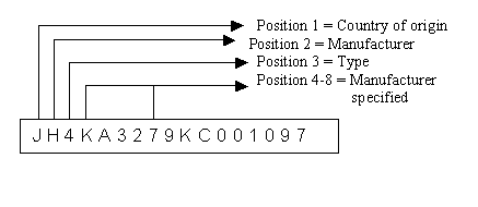
Figure 19.4
Lack of legacy standards
Items such as descriptions, names, labels and keys have typically been managed on an application-by-application basis. In many legacy systems, such fields lack clear definition. For example, data in the name field sometimes is haphazardly formatted (Brent Thomas; Elizabeth A. Hammergreen; and Herny, Ashley). Moreover, application software providers may offer user-oriented fields, which can be used and defined as required by the customer.
Non-centralised key data
As companies have evolved through acquisition or growth, various systems have taken ownership of data that may not have been in their scope. This is especially true for companies that can be characterised as heavy users of packaged application software and those that have grown through acquisition. Notice how the non-centralised cust_no field varies from one database to another for a hypothetical company represented below:
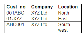
Figure 19.5
The ultimate goal of a transformation architecture is to allow the developers to create a repeatable transformation process. You should make sure to clearly define your needs for data synchronisation and data cleansing.
As a summary of the data architecture design, this section lists the main requirements placed on a data warehouse.
Subject-oriented data: Data that is contained within a data warehouse should be organised by subject. For example, if your data warehouse focuses on sales and marketing processes, you need to generate data about customers, prospects, orders, products, and so on. To completely define a subject area, you may need to draw upon data from multiple operational systems. To derive the data entities that clearly define the sales and marketing process of an enterprise, you might need to draw upon an order entry system, a sales force automation system, and various other applications.
Time-based data: Data in a data warehouse should relate specifically to a time period, allowing users to capture data that is relevant to their analysis period. Consider an example in which a new customer was added to an order entry system with a primary contact of John Doe on 2/11/99. This customer’s data was changed on 4/11/99 to reflect a new primary contact of Jane Doe. In this scenario, the data warehouse would contain the two contact records shown in the following table:
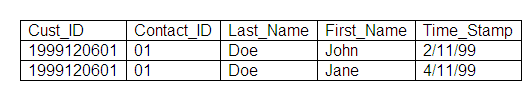
Figure 19.6
Update processing: A data warehouse should contain data that represents closed operational items, such as fulfilled customer order. In this sense, the data warehouse will typically contain little or no update processing. Typically, incremental or mass loading processes are run to insert data into the data warehouse. Updating individual records that are already in the data warehouse will rarely occur.
Transformed and scrubbed data: Data that is contained in a data warehouse should be transformed, scrubbed and integrated into user-friendly subject areas.
Aggregation: Data needs to be aggregated into and out of a data warehouse. Thus, computational requirements will be placed on the entire data warehousing process.
Granularity: A data warehouse typically contains multiple levels of granularity. It is normal for the data warehouse to be summarised and contain less detail than the original operational data; however, some data warehouses require dual levels of granularity. For example, a sales manager may need to understand how sales representatives in his or her area perform a forecasting task. In this example, monthly summaries that contain the data associated with the sales representatives’ forecast and the actual orders received are sufficient; there is no requirement to see each individual line item of an order. However, a retailer may need to wade through individual sales transactions to look for correlations that may show people tend to buy soft drinks and snacks together. This need requires more details associated with each individual purchase. The data required to fulfil both of these requests may exist, and therefore, the data warehouse might be built to manage both summarised data to fulfil a very rapid query and the more detailed data required to fulfil a lengthy analysis process.
Metadata management: Because a data warehouse pools information from a variety of sources and the data warehouse developers will perform data gathering on current data stores and new data stores, it is required that storage and management of metadata be effectively done through the data warehouse process.
An application architecture determines how users interact with a data warehouse. To determine the most appropriate application architecture for a company, the intended users and their skill levels should be assessed. Other factors that may affect the design of the architecture include technology currently available and budget constraints. In any case, however, the architecture must be defined logically rather than physically. The classification of users will help determine the proper tools to satisfy their reporting and analysis needs. A sampling of user category definitions is listed below:
Power users: Technical users who require little or no support to develop complex reports and queries. This type of user tends to support other users and analyse data through the entire enterprise.
Frequent users: Less technical users who primarily interface with the power users for support, but sometimes require the IT department to support them. These users tend to provide management reporting support up to the division level within an enterprise, a narrower scope than for power users.
Casual users: These users touch the system and computers infrequently. They tend to require a higher degree of support, which normally includes building predetermined reports, graphs and tables for their analysis purpose.
Tools must be made available to users to access a data warehouse. These tools should be carefully selected so that they are efficient and compatible with other parts of the architecture and standards.
Executive information systems (EIS): As mentioned earlier, these tools transform information and present that information to users in a meaningful and usable manner. They support advanced analytical techniques and free-form data exploration, allowing users to easily transform data into information. EIS tools tend to give their users a high-level summarisation of key performance measures to support decision-making. These tools fall into the big-button syndrome, in which an application development team builds a nice standard report with hooks to many other reports, then presents this information behind a big button. When a user clicks the button, magic happens.
Decision support systems (DSS): DSS tools are intended for more technical users, who require more flexibility and ad hoc analytical capabilities. DSS tools allow users to browse their data and transform it into information. They avoid the big button syndrome.
Ad hoc query and reporting: The purpose of EIS and DSS applications is to allow business users to analyse, manipulate and report on data using familiar, easy-to-use interfaces. These tools conform to presentation styles that business people understand and with which they are comfortable. Unfortunately, many of these tools have size restrictions that do not allow them to access large stores or to access data in a highly normalised structure, such as a Relational database, in a rapid fashion; in other words, they can be slow. Thus, users need tools that allow for more traditional reporting against Relational, or two-dimensional, data structures. These tools offer database access with limited coding and often allow users to create read-only applications. Ad hoc query and reporting tools are an important component within a data warehouse tool suite. Their greatest advantage is contained in the term 'ad hoc'. This means that decision makers can access data in an easy and timely fashion.
Production report writer: A production report writer allows the development staff to build and deploy reports that will be widely exploited by the user community in an efficient manner. These tools are often components within fourth generation languages (4GLs) and allow for complex computational logic and advanced formatting capabilities. It is best to find a vendor that provides an ad hoc query tool that can transform itself into a production report writer.
Application development environments (ADE): ADEs are nothing new, and many people overlook the need for such tools within a data warehouse tool suite. However, you will need to develop some presentation system for your users. The development, though minimal, is still a requirement, and it is advised that data warehouse development projects standardise on an ADE. Example tools include Microsoft Visual Basic and Powersoft Powerbuilder. Many tools now support the concept of cross-platform development for environment such as Windows, Apple Macintosh and OS/2 Presentation Manager. Every data warehouse project team should have a standard ADE in its arsenal.
Other tools: Although the tools just described represent minimum requirements, you may find a need for several other speciality tools. These additional tools include OLAP, data mining and managed query environments.
It is in the technology architecture section of the blueprint that hardware, software and network topology are specified to support the implementation of the data warehouse. This architecture is composed of three major components - clients, servers and networks – and the software to manage each of them.
Clients: The client technology component comprises the devices that are utilised by users. These devices can include workstations, personal computers, personal digital assistants and even beepers for support personnel. Each of these devices has a purpose being served by a data warehouse. Conceptually, the client either contains software to access the data warehouse (this is the traditional client in the client-server model and is known as a fat client), or it contains very little software and accesses a server that contains most of the software required to access a data warehouse. The later approach is the evolving Internet client model, known as a thin client and fat server.
Servers: The server technology component includes the physical hardware platforms as well as the operating systems that manage the hardware. Other components, typically software, can also be grouped within this component, including database management software, application server software, gateway connectivity software, replication software and configuration management software.
Networks: The network component defines the transport technologies needed to support communication activities between clients and servers. This component includes requirements and decisions for wide area networks (WANs), local area networks (LANs), communication protocols and other hardware associated with networks, such as bridges, routers and gateways.
Review question 3
What are the problems that you may encounter in the process of data cleansing?
Describe the three components of the technology architecture of a data warehousing system.
Data warehouses can best be modelled using a technique known as star schema modelling. It defines data entities in a way that supports the decision-makers’ view of a business and that reflects the important operational aspects of the business. A star schema contains three logical entities: dimension, measure and category detail (or category for short).
A star schema is optimised to queries, and therefore provides a database design that is focused on rapid response to users of the system. Also, the design that is built from a star schema is not as complicated as traditional database designs. Hence, the model will be more understandable for users of the system. Also, users will be able to better understand the navigation paths available to them through interpreting the star schema. This logical database design’s name hails from a visual representation derived from the data model: it forms a star, as shown below:
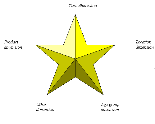
Figure 19.7
The star schema defines the join paths for how users access the facts about their business. In the figure above, for example, the centre of the star could represent product sales revenues that could have the following items: actual sales, budget and sales forecast. The true power of a star schema design is to model a data structure that allows filtering, or reduction in result size, of the massive measure entities during user queries and searches. A star schema also provides a usable and understandable data structure, because the points of the star, or dimension entities, provide a mechanism by which a user can filter, aggregate, drill down, and slice and dice the measurement data in the centre of the star.
A star schema, like the data warehouse it models, contains three types of logical entities: measure, dimension and category detail. Each of these entities is discussed separately below.
Within a star schema, the centre of the star – and often the focus of the users’ query activity – is the measure entity. A measure entity is represented by a rectangle and is placed in the centre of a star schema diagram.
A sample of raw measure data is shown below:
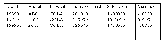
Figure 19.8
The data contained in a measure entity is factual information from which users derive 'business intelligence'. This data is therefore often given synonymous names to measure, such as key business measures, facts, metrics, performance measures and indicators. The measurement data provides users with quantitative data about a business. This data is numerical information that the users desire to monitor, such as dollars, pounds, degrees, counts and quantities. All of these categories allow users to look into the corporate knowledge base and understand the good, bad and ugly of the business process being measured.
The data contained within measure entities grows large over time, and therefore is typically of greatest concern to the technical support personnel, database administrators and system administrators.
Dimension entities are graphically represented by diamond-shaped squares, and placed at the points of the star. Dimension entities are much smaller entities compared with measure entities. The dimensions and their associated data allow users of a data warehouse to browse measurement data with ease of use and familiarity. These entities assist users in minimising the rows of data within a measure entity and in aggregating key measurement data. In this sense, these entities filter data or force the server to aggregate data so that fewer rows are returned from the measure entities. With a star schema model, the dimension entities are represented as the points of the star, as demonstrated in the diagram below, by the time, location, age group, product and other dimensions:
Figure 19.9
The diagram below illustrates an example of dimension data and a hierarchy representing the contents of a dimension entity:
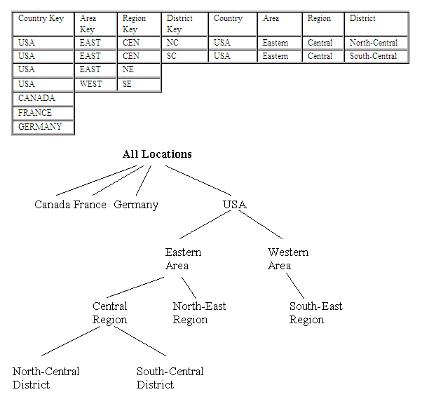
Figure 19.10
Each cell in a dimension is a category and represents an isolated level within a dimension that might require more detailed information to fulfil a user’s requirement. These categories that require more detailed data are managed within category detail entities. These entities have textual information that supports the measurement data and provides more detailed or qualitative information to assist in the decision-making process. The diagram below illustrates the need for a client category detail entity within the All Clients dimension:
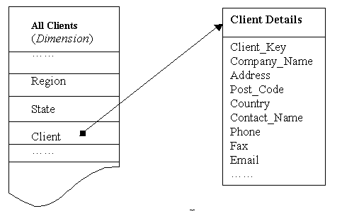
Figure 19.11
The stop sign symbol is usually used to graphically depict category entities, because users normally flow through the dimension entities to get the measure entity data, then stop their investigation with supporting category detail data.
During the data gathering process, an information package can be constructed, based on which star schema is formed. The table below shows an information package diagram ready for translation into a star schema. As can be seen from the table, there are six dimensions, and within each there are different numbers of categories. For example, the All Locations dimension has five categories while All Genders has one. The number within each category denotes the number of instances the category may have. For example, the All Time Periods will cover five different years with 20 quarters and 60 months. Gender will include male, female and unknown.
To define the logical measure entity, take the lowest category, or cell, within each dimension along with each of the measures and take them as the measure entity. For example, the measure entity translated from the table below would be Month, Store, Product, Age Group, Class and Gender with the measures Forecast Sales, Budget Sales, Actual Sales and Forecast Variance (calculated), and Budget Variance (calculated). They could be given a name Sales Analysis and put in the centre of the star schema in a rectangle.
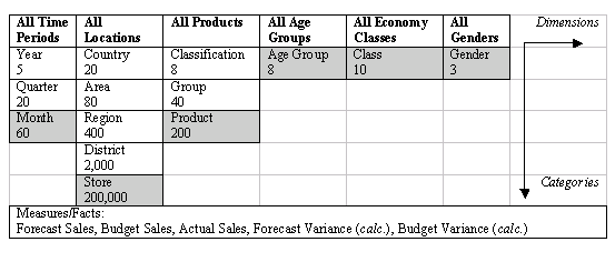
Figure 19.12
Each column of an information package in the table above defines a dimension entity and is placed on the periphery of the star of a star schema, symbolising the points of the star. Following the placement of the dimension entities, you want to define the relationships that they have with the measure entity. Because dimension entities always require representation within the measure entity, there always is a relationship. The relationship is defined over the lowest-level detail category for the logical model; that is, the last cell in each dimension. These relationships possess typically one-to-many cardinality; in other words, one dimension entity exists for many within the measures. For example, you may hope to make many product sales (Sales Analysis) to females (Gender) within the star model illustrated in the diagram below. In general, these relationships can be given an intuitive explanation such as: “Measures based on the dimension”. In the diagram below, for example, the relationship between Location (the dimension entity) and Sales Analysis (the measure entity) means “Sales Analysis based on Location”.
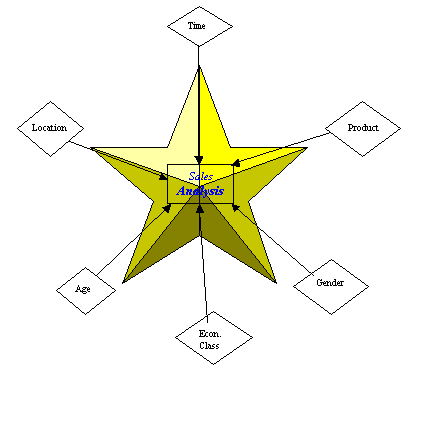
Figure 19.13
The final step in forming a star schema is to define the category detail entity. Each individual cell in an information package diagram must be evaluated and researched to determine if it qualifies as a category detail entity. If the user has a requirement for additional information about a category, this formulates the requirement for a category detail entity. These detail entities become extensions of dimension entities, as illustrated below:
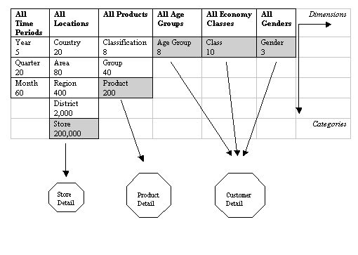
Figure 19.14
We need to know more detailed information about data such as Store, Product and customer categories (i.e. Age, Class and Gender). These detail entities (Store Detail, Product Detail and Customer Detail), having been added to the current star schema, now appear as shown below:
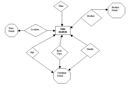
Figure 19.15
Review question 4
What are the three types of entities in a star schema and how are they used to model a data warehouse?
Exercise 1
An information package of a promotional analysis is shown below. To evaluate the effectiveness of various promotions, brand managers are interested in analysing data for the products represented, the promotional offers, and the locations where the promotions ran. Construct a star schema based on the information package diagram, and discuss how the brand manager or other analysts can use the model to evaluate the promotions.
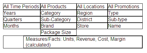
Figure 19.16
The construction of a data warehouse begins with careful considerations on architecture and data model issues, and with their sizing components. It is essential that a correct architecture is firmly in place, supporting the activities of a data warehouse. Having solved the architecture issue and built the data model, the developers of the data warehouse can decide what data they want to access, in which form, and how it will flow through an organisation. This phase of a data warehouse project will actually fill the warehouse with goods (data). This is where data is extracted from its current environment and transformed into the user-friendly data model managed by the data warehouse. Remember, this is a phase that is all about quality. A data warehouse is only as good as the data it manages.
The data extraction part of a data warehouse is a traditional design process. There is an obvious data flow, with inputs being operational systems and output being the data warehouse. However, the key to the extraction process is how to cleanse the data and transform it into usable information that the user can access and make into business intelligence.
Thus, techniques such as data flow diagrams may be beneficial for defining extraction specifications for the development. An important input for such a specification may be the useful reports that you collected during user interviews. In these kinds of reports, intended users often tell you what they want and what they do not, and then you can act accordingly.
Data needs to be processed for extraction and loading. An SQL select statement, shown below, is normally used in the process:
Select Target Column List
from Source Table List
where Join & Filter List
group by
or order by Sort & Aggregate List
Some complex extractions need to pull data from multiple systems and merge the resultant data while performing calculations and transformations for placement into a data warehouse. For example, the sales analysis example mentioned in the star schema modelling section might be such a process. We may obtain budget sales information from a budgetary system, which is different from the order entry system from which we get actual sales data, which in turn is different from the forecast management system from which we get forecast sales data. In this scenario, we would need to access three separate systems to fill one row within the Sales Analysis measure table.
Creating and defining a staging area can help the cleansing process. This is a simple concept that allows the developer to maximise up-time of a data warehouse while extracting and cleansing the data.
A staging area, which is simply a temporary work area, can be used to manage transactions that will be further processed to develop data warehouse transactions.
The concept of checkpoint restart has been around for many years. It originated in batch processing on mainframe computers. This type of logic states that if a long running process fails prior to completion, then restart the process at the point of failure rather than from the beginning. Similar logic should be implemented in the extraction and cleansing process. Within the staging area, define the necessary structures to monitor the activities of transformation procedures. Each of these programming units has an input variable that determines where in the process it should begin. Thus, if a failure occurs within the seventh procedure of an extraction process that has 10 steps, assuming the right rollback logic is in place, it would only require that the last four steps (7 through to 10) be conducted.
After data has been extracted, it is ready to be loaded into a data warehouse. In the data loading process, cleansed and transformed data that now complies with the warehouse standards is moved into the appropriate data warehouse entities. Data may be summarised and reformatted as part of this process, depending on the extraction and cleansing specifications and the performance requirements of the data warehouse. After the data has been loaded, data inventory information is updated within the metadata repository to reflect the activity that has just been completed.
Review question 5
How can a staging area help the cleansing process in developing a data warehousing system?
Why is checkpoint restart logic useful? How can it be implemented for the data extraction and cleansing process?
Data warehousing has been the subject of discussion so far. A data warehouse assembles data from heterogeneous databases so that users need only query a single system. The response to a user’s query depends on the contents of the data warehouse. In general, the warehouse system will answer the query as it is and will not attempt to extract further/implicit information from the data.
While a data warehousing system formats data and organises data to support management functions, data mining attempts to extract useful information as well as predicting trends and patterns from the data. Note that a data warehouse is not exclusive for data mining; data mining can be carried out in traditional databases as well. However, because a data warehouse contains quality data, it is highly desirable to have data mining functions incorporated in the data warehouse system. The relationship between warehousing, mining and database is illustrated below:
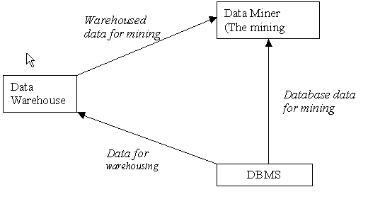
Figure 19.17
In general, a data warehouse comes up with query optimisation and access techniques to retrieve an answer to a query – the answer is explicitly in the warehouse. Some data warehouse systems have built-in decision-support capabilities. They do carry out some of the data mining functions, like predictions. For example, consider a query like “How many BMWs were sold in London in 2010”. The answer can clearly be in the data warehouse. However, for a question like “How many BMWs do you think will be sold in London in 2020”, the answer may not explicitly be in the data warehouse. Using certain data mining techniques, the selling patterns of BMWs in London can be discovered, and then the question can be answered.
Essentially, a data warehouse organises data effectively so that the data can be mined. As shown in in the diagram above, however, a good DBMS that manages data effectively could also be used as a mining source. Furthermore, data may not be current in a warehouse (it is mainly historical). If one needs up-to-date information, then one could mine the database, which also has transaction processing features. Mining data that keeps changing is often a challenge.
Data mining is a process of extracting previously unknown, valid and actionable information from large sets of data and then using the information to make crucial business decisions.
The key words in the above definition are unknown, valid and actionable. They help to explain the fundamental differences between data mining and the traditional approaches to data analysis, such as query and reporting and online analytical processing (OLAP). In essence, data mining is distinguished by the fact that it is aimed at discovery of information, without a previously formulated hypothesis.
First, the information discovered must have been previously unknown. Although this sounds obvious, the real issue here is that it must be unlikely that the information could have been hypothesised in advance; that is, the data miner is looking for something that is not intuitive or, perhaps, even counterintuitive. The further away the information is from being obvious, potentially the more value it has. A classic example here is the anecdotal story of the beer and nappies. Apparently a large chain of retail stores used data mining to analyse customer purchasing patterns and discovered that there was a strong association between the sales of nappies and beer, particularly on Friday evenings. It appeared that male shoppers who were out stocking up on baby requisites for the weekend decided to include some of their own requisites at the same time. If true, this shopping pattern is so counterintuitive that the chain’s competitors probably do not know about it, and the management could profitably explore it.
Second, the new information must be valid. This element of the definition relates to the problem of over optimism in data mining; that is, if data miners look hard enough in a large collection of data, they are bound to find something of interest sooner or later. For example, the potential number of associations between items in customers’ shopping baskets rises exponentially with the number of items. Some supermarkets have in stock up to 300,000 items at all times, so the chances of getting spurious associations are quite high. The possibility of spurious results applies to all data mining and highlights the constant need for post-mining validation and sanity checking.
Third, and most critically, the new information must be actionable. That is, it must be possible to translate it into some business advantage. In the case of the retail store manager, clearly he could leverage the results of the analysis by placing the beer and nappies closer together in the store or by ensuring that two items were not discounted at the same time. In many cases, however, the actionable criterion is not so simple. For example, mining of historical data may indicate a potential opportunity that a competitor has already seized. Equally, exploiting the apparent opportunity may require use of data that is not available or not legally usable.
Various applications may need data mining, but many of the problems have existed for years. Furthermore, data has been around for centuries. Why is it that we are talking about data mining now?
The answer to this is that we are using new tools and techniques to solve problems in a new way. We have large quantities of data computerised. The data could be in files, Relational databases, multimedia databases, and even on the World Wide Web. We have very sophisticated statistical analysis packages. Tools have been developed for machine learning. Parallel computing technology is maturing for improving performance. Visualisation techniques improve the understanding of the data. Decision support tools are also getting mature. Here are a few areas in which data mining is being used for strategic benefits:
Direct marketing: The ability to predict who is most likely to be interested in what products can save companies immense amounts in marketing expenditures. Direct mail marketers employ various data mining techniques to reduce expenditures; reaching fewer, better qualified potential customers can be much more cost effective than mailing to your entire mailing list.
Trend analysis: Understanding trends in the marketplace is a strategic advantage, because it helps reduce costs and timeliness to market. Financial institutions desire a quick way to recognise changes in customer deposit and withdraw patterns. Retailers want to know what product people are likely to buy with others (market basket analysis). Pharmaceuticals ask why someone buys their product over another. Researchers want to understand patterns in natural processes.
Fraud detection: Data mining techniques can help discover which insurance claims, cellular phone calls or credit card purchases are likely to be fraudulent. Most credit card issuers use data mining software to model credit fraud. Citibank, the IRS, MasterCard and Visa are a few of the companies who have been mentioned as users of such data mining technology. Banks are among the earliest adopters of data mining. Major telecommunications companies have an effort underway to model and understand cellular fraud.
Forecasting in financial markets: Data mining techniques are extensively used to help model financial markets. The idea is simple: if some trends can be discovered from historical financial data, then it is possible to predict what may happen in similar circumstances in the future. Enormous financial gains may be generated this way.
Mining online: Web sites today find themselves competing for customer loyalty. It costs little for customer to switch to competitors. The electronic commerce landscape is evolving into a fast, competitive marketplace where millions of online transactions are being generated from log files and registration forms every hour of every day, and online shoppers browse by electronic retailing sites with their finger poised on their mouse, ready to buy or click on should they not find what they are looking for - that is, should the content, wording, incentive, promotion, product or service of a Web site not meet their preferences. In such a hyper-competitive marketplace, the strategic use of customer information is critical to survival. As such, data mining has become a mainstay in doing business in fast-moving crowd markets. For example, Amazon, an electronics retailer, is beginning to want to know how to position the right products online and manage its inventory in the back-end more effectively.
End-users are often confused about the differences between query tools, which allow end-users to ask questions of a database management system, and data mining tools. Query tools do allow users to find out new and interesting facts from the data they have stored in a database. Perhaps the best way to differentiate these tools is to use an example.
With a query tool, a user can ask a question like: What is the number of white shirts sold in the north versus the south? This type of question, or query, is aimed at comparing the sales volumes of white shirts in the north and south. By asking this question, the user probably knows that sales volumes are affected by regional market dynamics. In other words, the end-user is making an assumption.
A data mining process tackles the broader, underlying goal of a user. Instead of assuming the link between regional locations and sales volumes, the data mining process might try to determine the most significant factors involved in high, medium and low sales volumes. In this type of study, the most important influences of high, medium and low sales volumes are not known. A user is asking a data mining tool to discover the most influential factors that affect sales volumes for them. A data mining tool does not require any assumptions; it tries to discover relationships and hidden patterns that may not always be obvious.
Many query vendors are now offering data mining components with their software. In future, data mining will likely be an option for all query tools. Data mining discovers patterns that direct end-users toward the right questions to ask with traditional queries.
Let’s review the concept of online analytical processing (OLAP) first. OLAP is a descendant of query generation packages, which are in turn descendants of mainframe batch report programs. They, like their ancestors, are designed to answer top-down queries from the data or draw what-if scenarios for business analysts. During the last decade, OLAP tools have grown popular as the primary methods of accessing database, data marts and data warehouses. OLAP tools are designed to get data analysts out of the custom report-writing business and into the 'cube construction' business. OLAP tools provide multidimensional data analysis – that is, they allow data to be broken down and summarised by product line and marketing region, for example.
OLAP deals with the facts or dimensions typically containing transaction data relating to a firm’s products, locations and times. Each dimension can also contain some hierarchy. For example, the time dimension may drill down from year, to quarter, to month, and even to weeks and days. A geographical dimension may drill up from city, to state, to region, to country and so on. The data in these dimensions, called measures, is generally aggregated (for example, total or average sales in pounds or units).
The methodology of data mining involves the extraction of hidden predictive information from large databases. However, with such a broad definition as this, an OLAP product could be said to qualify as a data mining tool. That is where the technology comes in, because for true knowledge discovery to take place, a data mining tool should arrive at this hidden information automatically.
Still another difference between OLAP and data mining is how the two operate on the data. Similar to the direction of statistics, OLAP is a top-down approach to data analysis. OLAP tools are powerful and fast tools for reporting on data, in contrast to data mining tools that focus on finding patterns in data. For example, OLAP involves the summation of multiple databases into highly complex tables; OLAP tools deal with aggregates and are basically concerned with addition and summation of numeric values, such as total sales in pounds. Manual OLAP may be based on need-to-know facts, such as regional sales reports stratified by type of businesses, while automatic data mining is based on the need to discover what factors are influencing these sales.
OLAP tools are not data mining tools since the query originates with the user. They have tremendous capabilities for performing sophisticated user-driven queries, but they are limited in their capability to discover hidden trends and patterns in database. Statistical tools can provide excellent features for describing and visualising large chunks of data, as well as performing verification-driven data analysis. Autonomous data mining tools, however, based on Artificial Intelligence (AI) technologies, are the only tools designed to automate the process of knowledge discovery.
Data mining is data-driven or discovery-driven analysis and requires no assumptions. Rather, it identifies facts or conclusions based on patterns discovered. OLAP and statistics provide query-driven, user-driven or verification-driven analysis. For example, OLAP may tell a bookseller about the total number of books it sold in a region during a quarter. Statistics can provide another dimension about these sales. Data mining, on the other hand, can tell you the patterns of these sales, i.e. factors influencing the sales.
Every time you visit a Web site, the Web server enters a valuable record of that transaction in a log file. Every time you visit an electronic commerce site, a cookie is issued to you for tracking what your interests are and what products or services you are purchasing. Every time you complete a form on a site, that information is written to a file. Although these server log files and form-generated databases are rich in information, the data is itself usually abbreviated and cryptic in plain text format with comma delimiters, making it difficult and time-consuming to mine. The volume of information is also overwhelming: a one-megabyte log file typically contains 4,000 to 5,000 page requests. Web site analysis tools typically import the log file data into a built-in database, which in turn transforms the data into aggregate reports or graphs.
This information can be fine-tuned to meet the needs of different individuals. For example, a Web administrator may want to know about the clicks leading to documents and images, files, scripts and applets. A designer will want to know how visitors navigate the site and whether there are paths or points from which many visitors jump to another site. The marketing team will want to know the effectiveness of certain promotions. Advertisers and partners may be interested in the number of click-throughs your site has generated to their sites. Most Web site analysis tools provide answers to such questions as:
What are the most common paths to the most important pages on your site?
What keywords bring the most traffic to your site from search engines?
How many pages do visitors typically view on your site?
How many visitors are you getting from different parts of the world?
How much time do visitors spend on your site?
How many new users visit your site every month?
However, like statistical and OLAP tools, Web analysis tools are verification-driven. They emphasise aggregate counts and spatial views of website traffic over time, and are not easily able to discover hidden patterns, which could provide you with information like, what the visitors are really looking for. The current Web site analysis tools are very good at innovative data reporting via tables, charts and graphs.
A data mining tool does not replace a Web analysis tool, but it does give the Web administrator a lot of additional opportunities for answering some of the marketing and business questions. For example, imagine trying to formulate answers to questions such as:
What is an optional segmentation of my Web site visitors?
Who is likely to purchase my new online products and services?
What are the most important trends in my site visitors’ behaviour?
What are the characteristics or features of my most loyal online clients?
Theoretically, these questions could be answered with a Web analysis tool. For example, a Web administrator could try to define criteria for a customer profile and query the data to see whether they work or not. In a process of trial and error, a marketer could gradually develop enough intuitions about the distinguishing features of its predominant Web site customers, such as their gender, age, location, income levels, etc. However, in a dynamic environment such as the Web, this type of analysis is very time-consuming and subject to bias and error.
On the other hand, a data mining tool (such as a decision tree generator) that incorporates machine-learning technology could find a better answer automatically, in a much shorter time – typically within minutes. More importantly, this type of autonomous segmentation is unbiased and driven by data, not the analyst’s intuition. For example, using a data mining tool, a log file can be segmented into statistically significant clusters very quickly.
The most common types of data mining tasks, classified based on the kind of knowledge they are looking for, are listed as follows:
Classification: Data records are grouped into some meaningful subclasses. For example, suppose a car sales company has some information that all the people in its list who live in City X own cars worth more than 20K. They can then assume that even those who are not on their list, but live in City X, can afford to own cars costing more than 20K. This way, the company classifies the people living in City X.
Sequence detection: By observing patterns in the data, sequences are determined. Here is an example: after John goes to the bank, he generally goes to the grocery store.
Data dependency analysis: Potentially interesting dependencies, relationships or associations between data items are detected. For example, if people buy X, they tend to buy Y as well. We say there is an association between X and Y.
Deviation analysis: For example, John went to the bank on Saturday, but he did not go to the grocery store after that. Instead, he went to a football game. With this task, anomalous instances and discrepancies are found.
Data mining is an integration of multiple technologies. These include data management such as database management, data warehousing, statistics, machine learning and decision support, and other technologies such as visualisation and parallel computing. Many of these technologies have existed for many decades. The ability to manage and organise data effectively has played a major role in making data mining a reality.
Database management researchers are taking advantages of work on deductive and intelligent query processing for data mining. One of the areas of interest is to extend query processing techniques to facilitate data mining. Data warehousing is another key data management technology for integrating the various data sources and organising the data so that it can be effectively mined.
Researchers in statistical analysis are integrating their techniques with those of machine learning to develop more sophisticated statistical techniques for data mining. Various statistical analysis packages are now being marketed as data mining tools. There is some dispute over this. Nevertheless, statistics is a major area contributing to data mining.
Machine learning has been around for a while. The idea here is for the machine to learn various rules from the patterns observed and then apply these rules to solve new problems. While the principles used in machine learning and data mining are similar, data mining usually considers large quantities of data to mine. Therefore, integration of database management and machine learning techniques are needed for data mining.
Researchers from the computing visualisation field are approaching the area from another perspective. One of their focuses is to use visualisation techniques to aid the mining process. In other words, interactive data mining is a goal of the visualisation community.
Decision support systems are a collection of tools and processes to help managers make decisions and guide them in management - for example, tools for scheduling meetings and organising events.
Finally, researchers in high-performance computing are also working on developing appropriate algorithms in order to make large-scale data mining more efficient and feasible. There is also interaction with the hardware community so that appropriate architectures can be developed for high-performance data mining.
While significant progresses have been made, there are still many challenges. For example, due to the large volumes of data, how can the algorithms determine which technique to select and what type of data mining to do? Furthermore, the data may be incomplete and/or inaccurate. At times, there may be redundant information, and at times there may not be sufficient information. It is also desirable to have data mining tools that can switch to multiple techniques and support multiple outcomes. Some of the current trends in data mining are illustrated below:
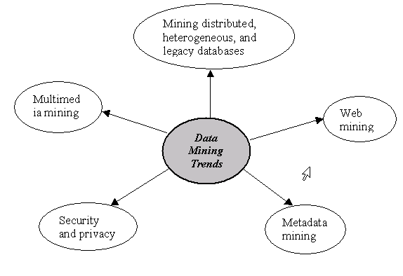
Figure 19.18
Review question 6
What is data mining? How is it used in the business world?
In general, when people talk about data mining, they focus primarily on the actual mining and discovery aspects. The idea sounds intuitive and attractive. However, mining data is only one step in the overall process. The diagram below illustrates the process as a multistep, iterative process:
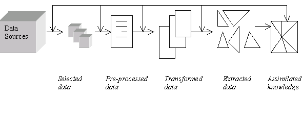
Figure 19.19
The business objectives drive the entire data mining process. They are the basis on which the initial project is established and the measuring stick by which the final results will be judged, and they should constantly guide the team throughout the process. Also, the process is highly iterative, with possibly many loop-backs over one or more steps. In addition, the process is far from autonomous. In spite of recent advances in technology, the whole data mining process remains very much a labour-intensive exercise.
However, not all steps are of equal weight in terms of typical time and effort spent. 60% of the time goes into preparing the data for mining, highlighting the critical dependency on clean, relevant data. The actual mining step typically constitutes about 10% of the overall effort.
This step in the data mining process has a lot in common with the initial step of any significant project undertaking. The minimum requirements are a perceived business problem or opportunity and some level of executive sponsorship. The first requirement ensures that there is a real, critical business issue that is worth solving, and the second guarantees that there is the political will to do something about it when the project delivers a proposed solution.
Frequently, you hear people saying: “Here is the data, please mine it.” But how do you know whether a data mining solution is really needed? The only way to find out is to properly define the business objectives. Ill-defined projects are not likely to succeed or result in added value. Developing an understanding and careful definition of the business needs is not a straightforward task in general. It requires the collaboration of the business analyst with domain knowledge and the data analyst, who can begin to translate the objectives into a data mining application.
This step in the process is also the time at which to start setting expectations. Nothing kills an otherwise successful project as quickly as overstated expectations of what could be delivered. Managing expectations will help to avoid any misunderstanding that may arise as the process evolves, and especially as the final results begin to emerge.
This is the most resource-consuming step in the process, typically requiring up to 60% of the effort of the entire project. The step comprises three phases:
Data selection: Identification and extraction of data.
Data pre-processing: Data sampling and quality testing.
Data transformation: Data conversion into an analytical model.
The goal of data selection is to identify the available data sources and extract the data that is needed for preliminary analysis in preparation for further mining. For example, if you want to find out who will respond to a direct marketing campaign, you need data (information) about customers who have previously responded to mailers. If you have their name and address, you should realise that this type of data is unique to a customer, and therefore, not the best data to be selected for mining. Information like city and area provides descriptive information, but demographic information is more valuable: items like a customer’s age, general income level, types of interests and household type.
Along with each of the selected variables, associated semantic information (metadata) is needed to understand what each of the variables means. The metadata must include not only solid business definitions of the data but also clear descriptions of data types, potential values, original source system, data formats and other characteristics. There are two major types of variables:
Categorical: The possible values are finite and differ in kind. For example, marital status (single, married, divorced, unknown), gender (male, female), customer credit rating (good, regular, poor).
Quantitative: There is measurable difference here between the possible values. There are two subtypes: continuous (values are real numbers) and discrete (values are integrates). Examples of continuous variables are income, average number of purchases and revenue. Examples of discrete variables are number of employees and time of year (month, season, quarter).
The variables selected for data mining are called active variables, in the sense that they are actively used to distinguish segments, make predictions or perform some other data mining operations.
When selecting data, another important consideration is the expected period of validity of the data. That is, the extent to which ongoing changes in external circumstances may limit the effectiveness of the mining. For example, because a percentage of customers will change their jobs every year, any analysis where job type is a factor has to be re-examined periodically.
At this stage, the data analyst has already begun to focus on the data mining algorithms that will best match the business application. This is an important aspect to keep in mind as the other phases of the data preparation step evolve, because it will guide the development of the analytical model and the fine-tuning of the data input.
The aim of data pre-processing is to ensure the quality of the selected data. Clean and well-understood data is a clear prerequisite for successful data mining, just as it is with other quantitative analysis. In addition, by getting better acquainted with the data at hand, you are more likely to know where to look for the real knowledge during the mining stage.
Without a doubt, data pre-processing is the most problematic phase in the data preparation step, principally because most operational data is never meant to be for data mining purposes. Poor data quality and poor data integrity are major issues in almost all data mining projects.
Normally, the data pre-processing phase begins with a general review of the structure of the data and some measuring of its quality. Such an approach usually involves a combination of statistical methods and data visualisation techniques. Representative sampling of the selected data is a useful technique, as large data volumes would otherwise make the review process very time-consuming.
For categorical variables, frequency distributions of the values are a useful way of better understanding the data content. Simple graphical tools such as histograms and pie charts can quickly plot the contribution made by each value for the categorical variable, and therefore help to identify distribution skews and invalid or missing values. One thing that must be noted is that the frequency distribution of any data should be considered based on a large enough representation sample. For example, if a set has 1 million males and 1 female, then it is not a valid study for females.
When dealing with quantitative variables, the data analyst is interested in such measures as maxim and minima, mean, mode (most frequently occurring value), median (midpoint value) and several statistical measures of central tendency; that is, the tendency for values to cluster around the mean. When combined, these measures offer a powerful way of determining the presence of invalid and skewed data. For example, maxim and minima quickly show up spurious data values, and the various statistical distribution parameters give useful clues about the level of noise in data.
During data pre-processing, two of the most common issues are noisy data and missing values.
Noisy data
With noisy data, one or more variables have values that are significantly out of line with what is expected for those variables. The observations in which these noisy values occur are called outliers. Outliers can indicate good news or bad – good news in the sense that they represent precisely the opportunities that we are looking for; bad news in that they may well be no more than invalid data.
Different kinds of outliers must be treated in different ways. One kind of outlier may be the result of a human error. For example, a person’s age is recorded as 650, or an income is negative. Clearly, these values have to be either corrected (if a valid value or reasonable substitution can be found) or dropped from the analysis. Another kind of outlier is created when changes in operational systems have not yet been reflected in the data mining environment. For example, new product codes introduced in operational systems show up initially as outliers. Clearly in this case, the only action required is to update the metadata.
Skewed distribution often indicates outliers. For example, a histogram may show that most of the people in the target group have low incomes and only a few are high earners. It may be that these outliers are good, in that they represent genuine high earners in this homogeneous group, or it may be that they result from poor data collection. For example, the group may consist mainly of retired people but, inadvertently, include a few working professionals.
In summary, what you do with outliers depends on their nature. You have to distinguish the good outlier from the bad and react appropriately.
Missing values
Missing values include values that are simply not present in the selected data, and/or those invalid values that we may have deleted during noise detection. Values may be missing because of human error; because the information was not available at the time of input; or because the data was selected across heterogeneous sources, thus creating mismatches. To deal with missing values, data analysts use different techniques, none of which is ideal.
One technique is simply to eliminate the observations that have missing values. This is easily done, but it has the obvious drawback of losing valuable information. Although this data loss may be less of a problem in situations where data volumes are large, it certainly will affect results in mining smaller volumes or where fraud or quality control is the objective. In these circumstances, we may well be throwing away the very observations for which we are looking. Indeed, the fact that the value is missing may be a clue to the source of the fraud or quality problem. If there is a large number of observations with missing values for the same variable, it may be an option to drop the variable from the analysis. This again has serious consequences because, unknown to the analyst, the variable may have been a key contributor to the solution.
The decision to eliminate data is never an easy one, nor can the consequences be easily foreseen. Luckily, there are several ways around the problem of missing values. One approach is to replace the missing value with its most likely value. For quantitative variables, this most likely value could be the mean or mode. For categorical variables, this could be the mode or a newly created value for the variable, called UNKNOWN, for example. A more sophisticated approach for both quantitative and categorical variables is to use a predictive model to predict the most likely value for a variable, on the basis of the values of other variables in observation.
Despite this stockpile of weapons to combat the problem of missing data, you must remember that all this averaging and predicting comes at a price. The more guessing you have to do, the further away from the real data the database moves. Thus, in turn, it can quickly begin to affect the accuracy and validation of the mining results.
During data transformation, the pre-processed data is transformed to produce the analytical data model. The analytical data model is an informational data model, and it represents a consolidated, integrated and time-dependent restructuring of the data selected and pre-processed from various operational and external sources. This is a crucial phase, as the accuracy and validity of the final results depend vitally on how the data analyst decides to structure and present the input. For example, if a department store wants to analyse customer spending patterns, the analyst must decide whether the analysis is to be done at some overall level, at the department level, or at the level of individual purchased articles. Clearly, the shape of the analytical data model is critical to the types of problems that the subsequent data mining can solve.
After the model is built, the data is typically further refined to suit the input format requirements of the particular data mining algorithm to be used. The fine-tuning typically involves data recording and data format conversion and can be quite time-consuming. The techniques used can range from simple data format conversion to complex statistical data reduction tools. Simple data conversions can perform calculations such as a customer’s age based on the variable of the date of birth in the operational database. It is quite common to derive new variables from original input data. For example, a data mining run to determine the suitability of existing customers for a new loan product might require to input the average account balance for the last 3-, 6- and 12-month periods.
Another popular type of transformation is data reduction. Although it is a general term that involves many different approaches, the basic objective is to reduce the total number of variables for processing by combining several existing variables into one new variable. For example, if a marketing department wants to gauge how attractive prospects can be for a new, premium-level product, it can combine several variables that are correlated, such as income, level of education and home address, to derive a single variable that represents the attractiveness of the prospect. Reducing the number of input variables produces a smaller and more manageable set for further analysis. However, the approach has several drawbacks. It is not always easy to determine which variables can be combined, and combining variables may cause some loss of information.
Clearly, data remodelling and refining are not trivial tasks in many cases, which explains the amount of time and effort that is typically spent in the data transformation phase of the data preparation step.
Another technique, called discretisation, involves converting quantitative variables into categorical variables, by dividing the values of the input variables into buckets. For example, a continuous variable such as income could be discretised into a categorical variable such as income range. Incomes in the range of £0 to £15,000 could be assigned a value Low; those in the range of £15,001 to £30,000 could be assigned a value Medium, and so on.
Last, One-of-N is also a common transformation technique that is useful when the analyst needs to convert a categorical variable to a numeric representation, typically for input to a neural network. For example, a categorical variable - type of car - could be transformed into a quantitative variable with a length equal to the number of different possible values for the original variable, and having an agreed coding system.
At last we come to the step in which the actual data mining takes place. The objective is clearly to apply the selected data mining algorithm(s) to the pre-processed data.
In reality, this step is almost inseparable from the next step (analysis of results) in this process. The two are closely inter-linked, and the analyst typically iterates around the two for some time during the mining process. In fact, this iteration often requires a step back in the process to the data preparation step. Two steps forward, one step back often describes the reality of this part of the data mining process.
What happens during the data mining step is dependent on the type of application that is under development. For example, in the case of a database segmentation, one or two runs of the algorithm may be sufficient to clear this step and move into analysis of results. However, if the analyst is developing a predictive model, there will be a cyclical process where the models are repeatedly trained and retrained on sample data before being tested against the real database. Data mining developments typically involve the use of several algorithms, which will be discussed in a later part of the chapter.
Needless to say, analysing the results of the mining run is one of the most important steps of the whole process. In addition, in spite of improvements in graphical visualisation aids, this step can only be done properly by a skilled data analyst working with a business analyst. The analysis of results is inseparable from the data mining step in that the two are linked in an interactive process.
The specific activities in this step depend very much on the kind of application that is being developed. For example, when performing a customer database segmentation, the data analyst and business analyst attempt to label each of the segments, to put some business interpretation on them. Each segment should be homogeneous enough to allow for this. However, if there are only a few segments with large concentrations of customer records, the segment cannot be sufficiently differentiated. In this case, changing the variables on which the segmentation is based improves the result. For example, removing the most common variables from the large segments gives a more granular segmentation on a rerun.
When predictive models are being developed, a key objective is to test their accuracy. This involves comparing the prediction measures against known actual results, and input sensitivity analyses (the relative importance attributed to each of the input variables). Failure to perform satisfactorily usually guides the team toward the unduly influential input, or sends it in search of new input variables. One common source of error when building a predictive model is the selection of overly predictive variables. In the worst case, the analyst may inadvertently select a variable that is recorded only when the event that he or she is trying to predict occurs. Take, for example, policy cancellation data as input to a predictive model for customer attrition. The model will perform with 100% accuracy, which should be a signal to the team to recheck the input.
Another difficulty in predictive modelling is that of over-training, where the model predicts well on the training data but performs poorly on the unseen test data. The problem is caused by over-exposure to the training data – the model learns the detailed patterns of that data but cannot generalise well when confronted with new observations from the test data set.
Developing association rules also poses special considerations. For example, many association rules discovered may be inactionable or will reflect no more than one-off instances. In some other cases, only the major rules, which are already well known and therefore not actionable, are discovered. Clearly, this is one area where careful tuning and iteration are needed to derive useful information.
This step closes the loop, which was opened when we set the business objectives at the beginning of the process. The objective now is to put into action the commitments made in that opening step, according to the new, valid and actionable information from the previous process steps. There are two main challenges in this step: to present the new findings in a convincing, business-oriented way, and to formulate ways in which the new information can be best exploited.
Several technical issues need to be considered. At a minimum, the new information may manifest itself as new data mining applications or modifications to be integrated into existing technical infrastructure. Integration could involve the inclusion of new predictive models and association rules in existing application code, expert system shells or database procedures. In addition, operational and informational system databases may be enhanced with new data structures. In any event, the experiences during the data preparation step will doubtless put a focus on data integrity in upstream operational systems. This focus will create a demand for improved data quality and documentation in these systems, and improved manual procedures to prevent error or fraud.
There exist a large number of different approaches to data mining, and they can be confusing initially. One reason for such confusions might be that inconsistent terminology is used among data mining practitioners themselves. The table below offers some examples of data mining applications, together with their supporting operations (models) and techniques (algorithms):
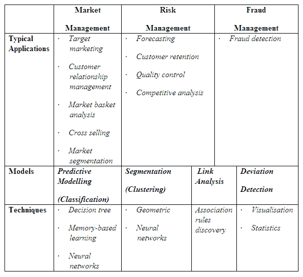
Figure 19.20
The applications listed in the table represent typical business areas where data mining is used today. Predictive modelling, database segmentation, link analysis and deviation detection are the four major operations or models for implementing any of the business applications. We deliberately do not show a fixed, one-to-one link between the applications and data mining model layers, to avoid suggestions that only certain models are appropriate for certain applications and vice versa. Nevertheless, certain well-established links between the applications and the corresponding operation models do exist. For example, target marketing strategies are always implemented by means of the database segmentation operation. In addition, the operations (models) are not mutually exclusive. For example, a common approach to customer retention is to segment the database first and then apply predictive modelling to the resultant, more homogeneous segments.
Decision trees (or a series of IF/THEN rules) as a commonly used machine learning algorithm are powerful and popular tools for classification and prediction. They normally work in supervised learning situations, where they attempt to find a test for splitting a database among the most desired categories, such as “Web site visitor will buy vs. will not buy”. In both instances, these algorithms will try to identify important data clusters of features within a database. Normally, an attribute (feature/field) is tested at a node of a tree; the number of branches from that node is usually the number of possible values of that attribute (for example, for gender, it will be Male, Female or Unknown, so three branches for node gender). If the attribute is numeric, the node in a decision tree usually tests whether its value is less than a predetermined constant, giving a two-way split. Missing values in a data set are treated as an attribute value in their own right. Consideration is given to the fact that a missing value may be of some significance. An example of decision trees is shown below. It may be generated from past experience (data) and can be used to decide what to do according to weather conditions.
Data mining tools incorporating machine learning algorithms such as CART (classification and regression trees), CHAID (chi-squared automatic integration detection), ID3 (Interactive Dichotomizer) or C4.5 or C5.0 will segment a data set into statistically significant clusters of classes based on a desired output. Some of these tools generate 'decision trees' that provide a graphical breakdown of a data set, while others produce IF/THEN rules, which segment a data set into classes that can point out important ranges and features. Such a rule has two parts, a condition (IF) and a result (THEN), and is represented as a statement. For example:
IF customer_code is 03 AND number_of_purchases_made_this_year is 06 AND post_code is W1 THEN will purchase Product_X
Rule’s probability: 88%. The rule exists in 13000 records. Significance level: Error probability < 13%
A measure of information
There are two main types of decision trees: binary and multiple branches. A binary decision tree splits from a node in two directions, with each node representing a yes-or-no question like the tree below. Multiple-branched decision trees, on the other hand, can accommodate more complex questions with more than two answers. Also, a node in such a tree can represent an attribute with more than two possible values.
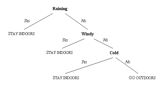
Figure 19.21
As mentioned before, there are a number of practical algorithms for building decision trees. ID3 is one of them - it can automatically build trees from given positive or negative instances. Each leaf of a decision tree asserts a positive or negative concept.
To classify a particular input, we start at the top and follow assertions down until we reach an answer. As an example, the following table lists the relationship between species of animals and their features such as diet, size, colour and habitat. Given a set of examples such as this, ID3 induces an optimal decision tree for classifying instances. As can be seen from the figure, not all of the features presented in the table are necessary for distinguishing classes. In this example, the size feature is not needed at all for classifying the animals. Similarly, once the brown or grey branches of the tree are taken, the remaining features can be ignored. It means that colour alone is sufficient to distinguish rabbits and weasels from the other animals.
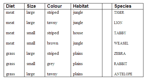
Figure 19.22
The ID3 algorithm builds a decision tree in which any classification can be performed by checking the fewest features (that is why the tree is called optimal). It builds the tree by first ranking all the features in terms of their effectiveness, from an information-theoretic standpoint, in partitioning the set of target classes. It then makes this feature the root of the tree; each branch represents a partition of the set of classifications. The algorithm then recurs on each branch with the remaining features and classes. When all branches lead to single classifications, the algorithm terminates.
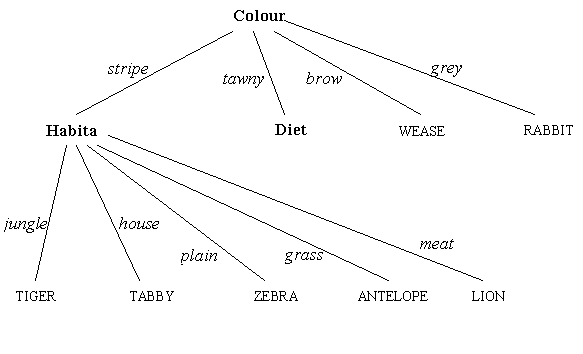
Figure 19.23
Neural networks (NN) are another popular data mining technique. An NN is a system of software programs and data structures that approximates the operation of the brain. It usually involves a large number of processors (also called elements/neurons/nodes) operating in parallel, each with its own small sphere of knowledge and access to data in its local memory. Typically, an NN is initially 'trained' or fed with large amounts of data and rules about data relationships. NNs are basically computing memories where the operations are all about association and similarity. They can learn when sets of events go together, such as when one product is sold, another is likely to sell as well, based on patterns they have observed over time.
This is basically how most neural networks learn: by example, in a supervised mode (the correct output is known and provided to the network). Supervised models, such as back propagation networks, are trained with pairs of examples: positive and negative. A given input pattern is matched with a desired output pattern. Training a supervised network is a process of providing a set of inputs and outputs, one at a time. The network trains by taking in each input pattern, producing an output pattern, and then comparing its output to the desired output. If the network output is different from the desired output, the network adjusts its internal connection strengths (weights) in order to reduce the difference between the actual output and the desired output. If, however, its output matches the desired output, then the network has learned the pattern and no correction is necessary. This process continues until the network gets the patterns of input/output correct or until an acceptable error rate is attained.
However, because the network may get one set of patterns correct and another wrong, the adjustments that it makes are continuous. For this reason, training of a network is an interactive process where input/output patterns are presented over and over again until the network 'gets' the patterns correctly.
A trained network has the ability to generalise on unseen data; that is, the ability to correctly assess samples that were not in the training data set. Once you train a network, the next step is to test it. Expose the network to samples it has not seen before and observe the network’s output. A common methodology is to split the available data, training on a portion of the data and testing on the rest.
In general, it is easier for a NN to learn a set of distinct responses (e.g. yes vs. no) than a continuous valued response (e.g. sales price). A common way to deal with this problem is to 'discrete' an attribute. Rather than having a single input for each sale amount, you might break it down to several ranges. Here is an example. Let’s say a Web site sells software products that range in price from very low to very high. Here, the 1-of-N coding conversion is adopted:
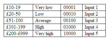
Figure 19.24
Most of today’s data mining tools are able to shift the data into these discrete ranges. You should make sure that you include all ranges of values for all the variables that the network is subject to encounter. In the Web site example, this means including the least and most expensive items, and the lowest and highest amounts of sales, session times, units sold, etc. As a rule, you should have several examples in the training set for each value of a categorical attribute and for a range of values for ordered discrete and continuous valued features.
As a summary of supervised NNs for data mining, the main tasks in using a NN tool are listed below:
Identify the input variables – this is very important.
Convert the variables into usable ranges – pick a tool which will do this.
Decide on the format of the output – continuous or categorical?
Decide on a set of training data samples and a training schedule.
Test the model and apply it in practice.
SOM networks are another type of popular NN algorithm that incorporate with today’s data mining tool. An SOM network resembles a collection of neurons, as in the human brain, each of which is connected to its neighbour. As an SOM is exposed to samples, it begins to create self-organising clusters, like cellophane spreading itself over chunks of data. Gradually, a network will organise clusters and can therefore be used for situations where no output or dependent variable is known. SOM has been used to discover associations for such purposes as market basket analysis in retailing.
The most significant feature of an SOM is that it involves unsupervised learning (using a training sample for which no output is known), and is commonly used to discover relations in a data set. If you do not know what you are attempting to classify, or if you feel there may be more than one way to categorise the data, you may want to start with an SOM.
Activity 2 – SOM neural networks
http://websom.hut.fi/websom/ is a site describing SOM networks for text mining. It provides good demonstration of the system. Try to see how text documents are clustered by SOM.
Review question 7
• What is a decision tree? Use an example to intuitively explain how it can be used for data mining.
• What are the differences between supervised and unsupervised learning?
In this chapter, we have covered the most important aspects of data warehousing and data mining. The following topics are open to discussion:
Data warehouse systems are so powerful – they improve data quality, allow timely access, support for organisational change, improve productivity and reduce expense. Why do we still need operational systems?
Discuss the relationships between database, data warehouse and data mining.
Discuss why data mining is an iterative process.